Model and source
- Citation: Savic RM, Mentre F, Lavielle M. (2011). Implementation and Evaluation of the SAEM Algorithm for Longitudinal Ordered Categorical Data with an Illustration in Pharmacokinetics-Pharmacodynamics. The AAPS Journal 13(1):44-53. doi:[10.1208/s12248-010-9238-5](https://doi.org/10.1208/s12248-010-9238-5).
- The model implemented here is the worked PKPD illustration from the paper’s “Illustration on Real Data” section (Page 6) – one-compartment oral PK with an absorption lag time, an effect compartment, and a proportional-odds (cumulative-logit) PD model on a three-category recoding of percent prothrombin complex activity (PCA).
- The paper’s primary contribution is the extension and Monte Carlo evaluation of the SAEM algorithm in MONOLIX 3.1 for ordered-categorical mixed-effects models (simulation Scenarios A-E against the Jonsson et al. 2004 NONMEM benchmark). The warfarin PKPD example is included as a worked demonstration of MONOLIX’s simultaneous continuous-plus-categorical fitting, not as a substantive warfarin popPK characterisation – see the Assumptions and deviations section below for the scope rationale.
Population
The PKPD dataset is the well-known historical warfarin set originally
described by O’Reilly and Aggeler (1968; Circulation 38:169) and
O’Reilly et al. (1963; J Clin Invest 42:1542) – references 16 and 17 in
Savic 2010. The Savic 2010 paper’s Page 6 wording is “33 patients … a
single dose of warfarin for 140 h post dose”, with 251 PK observations
and 232 PD observations available. The original O’Reilly cohort was
healthy adult volunteers studied at the San Francisco Veterans
Administration Medical Center; Savic 2010 does not re-document age,
weight, sex, race, or dose range and reports model parameters in
absolute units (V = 7.96 L; Cl = 0.132 L/h). The full population
metadata is available programmatically via
readModelDb("Savic_2010_warfarin")$population.
Source trace
The per-parameter origin is recorded as an in-file comment next to
each ini() entry in
inst/modeldb/specificDrugs/Savic_2010_warfarin.R. The table
below collects them in one place for review. Every parameter value in
the file is from Figure 4 of Savic 2010 (the MONOLIX output for the
real-data example).
| Equation / parameter | Value | Source location |
|---|---|---|
| PK structure (1-cmt + lag + effect cmt) | n/a | Page 6 prose; Page 8 Fig. 3 MONOLIX $ODE block |
| PD structure (proportional odds, cumulative logit on Ce) | n/a | Page 6 prose; Page 8 Fig. 3 MONOLIX $CATEGORICAL
block |
Tlag (absorption lag) |
0.9 h | Page 8 Fig. 4 row “Tlag : 0.9 (s.e. 0.19, r.s.e. 21)” |
ka (absorption rate) |
1.45 1/h | Page 8 Fig. 4 row “ka : 1.45 (s.e. 0.54, r.s.e. 37)” |
V (apparent central volume) |
7.96 L | Page 8 Fig. 4 row “V : 7.96 (s.e. 0.33, r.s.e. 4)” |
Cl (apparent clearance) |
0.132 L/h | Page 8 Fig. 4 row “Cl : 0.132 (s.e. 0.0067, r.s.e. 5)” |
ke0 (effect-compartment rate) |
0.0179 1/h | Page 8 Fig. 4 row “ke0 : 0.0179 (s.e. 0.001, r.s.e. 6)” |
alpha1 (cum-logit intercept for P(Y >= 2)) |
-10.5 | Page 8 Fig. 4 row “alpha1 : -10.5 (s.e. 1.6, r.s.e. 15)” |
alpha2 (cum-logit increment for P(Y >= 1)) |
5.41 | Page 8 Fig. 4 row “alpha2 : 5.41 (s.e. 0.92, r.s.e. 17)” |
beta (cum-logit slope on Ce) |
4.5 1/(mg/L) | Page 8 Fig. 4 row “beta : 4.5 (s.e. 0.56, r.s.e. 12)” |
| omega2_Tlag | 0.252 | Page 8 Fig. 4 row “omega2_Tlag : 0.252 (s.e. 0.15, r.s.e. 59)” |
| omega2_ka | 0.689 | Page 8 Fig. 4 row “omega2_ka : 0.689 (s.e. 0.46, r.s.e. 66)” |
| omega2_V | 0.0478 | Page 8 Fig. 4 row “omega2_V : 0.0478 (s.e. 0.013, r.s.e. 28)” |
| omega2_Cl | 0.0797 | Page 8 Fig. 4 row “omega2_Cl : 0.0797 (s.e. 0.021, r.s.e. 26)” |
| omega2_ke0 | 0.0229 | Page 8 Fig. 4 row “omega2_ke0 : 0.0229 (s.e. 0.02, r.s.e. 87)” |
| omega2_alpha1 | 8.74 | Page 8 Fig. 4 row “omega2_alpha1 : 8.74 (s.e. 4.3, r.s.e. 49)” |
Additive PK residual a
|
0.231 mg/L | Page 8 Fig. 4 row “a : 0.231 (s.e. 0.047, r.s.e. 20)” |
Proportional PK residual b
|
0.0632 | Page 8 Fig. 4 row “b : 0.0632 (s.e. 0.0092, r.s.e. 15)” |
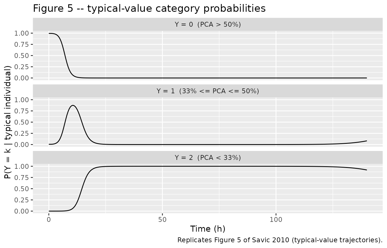
| PD categorisation (cutoffs 50% and 33% PCA) | n/a | Page 6 prose: “Y = 0 if PCA > 50%, Y = 1 if 33% <= PCA <= 50%, Y = 2 if PCA < 33%” |
Virtual cohort
Original observed data are not redistributed here. The simulations below use a 33-subject virtual cohort matched to the Savic 2010 illustration in size and dosing window. Savic 2010 does not report individual body weights; the parameters are reported in absolute units (V = 7.96 L, Cl = 0.132 L/h) rather than weight-normalised form, so the simulation does not scale by body weight. The dose used here is 100 mg (a single oral dose), which puts the typical peak central concentration near 13 mg/L (= 100 mg / 7.96 L), consistent with the observed peak in Savic 2010 Figure 1 (left panel).
Simulation
mod <- readModelDb("Savic_2010_warfarin")

sim <- rxode2::rxSolve(mod, events = events) |>
  as.data.frame() |>
  dplyr::rename(time_h = time)
#> ℹ parameter labels from comments will be replaced by 'label()'
For deterministic typical-value replication (Figure 5, below) the random effects are zeroed out and a single subject is simulated:
mod_typical <- mod |> rxode2::zeroRe()
#> ℹ parameter labels from comments will be replaced by 'label()'
events_typical <- rxode2::et(
  amt = dose_mg, cmt = "depot", evid = 1, time = 0
) |>
  rxode2::et(seq(0, sim_horizon_h, by = 0.5)) |>
  rxode2::et(id = 1L)

sim_typical <- rxode2::rxSolve(mod_typical, events = events_typical) |>
  as.data.frame() |>
  dplyr::rename(time_h = time)
#> ℹ omega/sigma items treated as zero: 'etaltlag', 'etalka', 'etalvc', 'etalcl', 'etalke0', 'etaalpha1'
Replicate published figures
Figure 1 (left panel) – observed PK
Savic 2010 Figure 1 left panel plots warfarin plasma concentration (mg/L) vs. time (h) across the 33-subject cohort. The simulated VPC below uses the IIV specification from Figure 4. Original-data digitisation is not attempted; the visual envelope of the simulated cohort is the comparison surface.
pk_summary <- sim |>
  dplyr::group_by(time_h) |>
  dplyr::summarise(
    Q05 = stats::quantile(Cc, 0.05, na.rm = TRUE),
    Q50 = stats::quantile(Cc, 0.50, na.rm = TRUE),
    Q95 = stats::quantile(Cc, 0.95, na.rm = TRUE),
    .groups = "drop"
  )

ggplot(pk_summary, aes(time_h, Q50)) +
  geom_ribbon(aes(ymin = Q05, ymax = Q95), alpha = 0.25) +
  geom_line() +
  labs(
    x = "Time (h)",
    y = "Warfarin plasma concentration Cc (mg/L)",
    title = "Figure 1 (left panel) -- typical PK VPC",
    caption = "Replicates Figure 1 left panel of Savic 2010."
  )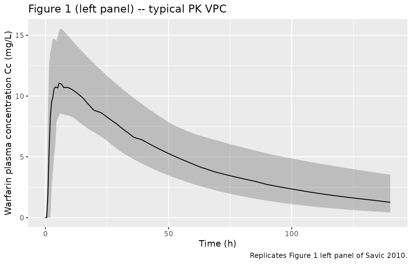
Figure 5 – typical-value category probabilities over time
Savic 2010 Figure 5 plots the typical-value probability of each warfarin response category (Y = 0, 1, 2) over time, from simulations of the final model. Here we replicate that figure by zeroing the random effects and plotting the derived states P_eq0, P_eq1, P_eq2.
prob_df <- sim_typical |>
  dplyr::select(time_h, P_eq0, P_eq1, P_eq2) |>
  tidyr::pivot_longer(
    cols      = c(P_eq0, P_eq1, P_eq2),
    names_to  = "category",
    values_to = "probability"
  ) |>
  dplyr::mutate(category = factor(
    category,
    levels = c("P_eq0", "P_eq1", "P_eq2"),
    labels = c("Y = 0  (PCA > 50%)", "Y = 1  (33% <= PCA <= 50%)", "Y = 2  (PCA < 33%)")
  ))

ggplot(prob_df, aes(time_h, probability)) +
  geom_line() +
  facet_wrap(~category, ncol = 1) +
  scale_y_continuous(limits = c(0, 1)) +
  labs(
    x = "Time (h)",
    y = "P(Y = k | typical individual)",
    title = "Figure 5 -- typical-value category probabilities",
    caption = "Replicates Figure 5 of Savic 2010 (typical-value trajectories)."
  )
PKNCA validation
Use PKNCA for Cmax, Tmax, AUC, and half-life of the simulated warfarin PK. The model is one-compartment oral with a lag time; the expected half-life is ln(2) / kel = ln(2) * V / Cl = ln(2) * 7.96 / 0.132 ~ 41.8 h, broadly consistent with the published warfarin terminal half-life of 36-42 h.
sim_nca <- sim |>
  dplyr::filter(!is.na(Cc)) |>
  dplyr::transmute(id = id, time = time_h, Cc = Cc, treatment = "single_oral")

conc_obj <- PKNCA::PKNCAconc(sim_nca, Cc ~ time | treatment + id)

dose_df <- data.frame(
  id        = seq_len(n_sub),
  time      = 0,
  amt       = dose_mg,
  treatment = "single_oral"
)

dose_obj <- PKNCA::PKNCAdose(dose_df, amt ~ time | treatment + id)

intervals <- data.frame(
  start      = 0,
  end        = Inf,
  cmax       = TRUE,
  tmax       = TRUE,
  aucinf.obs = TRUE,
  half.life  = TRUE
)

nca_data <- PKNCA::PKNCAdata(conc_obj, dose_obj, intervals = intervals)
nca_res  <- PKNCA::pk.nca(nca_data)

nca_summary <- summary(nca_res)
knitr::kable(nca_summary, caption = "Simulated NCA parameters for single 100 mg oral dose.")| start | end | treatment | N | cmax | tmax | half.life | aucinf.obs |
|---|---|---|---|---|---|---|---|
| 0 | Inf | single_oral | 33 | 11.4 [20.5] | 4.50 [2.00, 11.5] | 45.7 [16.0] | 764 [35.1] |
Comparison against published NCA
Savic 2010 does not tabulate Cmax, Tmax, AUC, or half-life as discrete outputs; the paper’s PK contribution is the parameter table in Figure 4 (MONOLIX output) rather than an NCA summary table. The simulated NCA above serves as a sanity check that the implemented PK structure reproduces a warfarin-like profile (long half-life around 40 h; Tmax in the first half-day; AUC scaled by clearance):
-
kel = Cl / V = 0.132 / 7.96 = 0.0166 1/himpliest_{1/2} = ln(2) / kel ~ 41.8 h. -
AUC_inf = Dose / Cl = 100 / 0.132 ~ 758 mg*h/Lfor a 100 mg dose. -
Cmaxat the absorption peak (around1 / ka + Tlag~ 1.6 h) sits nearDose / V = 100 / 7.96 ~ 12.6 mg/L, modulo the absorption-elimination exponential decay term.
Assumptions and deviations
PD categorisation caveat (load-bearing). The PD endpoint in Savic 2010 is a deliberate three-category recoding of the continuous PCA variable (Y = 0 if PCA > 50%; Y = 1 if 33% <= PCA <= 50%; Y = 2 if PCA < 33%). The authors explicitly write (Page 6): “categorization of the continuous variable is done for illustration purpose only, and it is not recommended to be done in the real analysis.” The cutoffs (50%, 33%) were chosen to approximate INR clinical-target ranges (low INR < 2 maps to category 0; targeted INR 2-3 maps to category 1; high INR > 3 maps to category 2). The model is an instructive demonstration of the SAEM algorithm’s simultaneous continuous-plus-discrete-data capability and is not intended as a clinical warfarin PKPD characterisation. Users who need a continuous-PCA warfarin PKPD model should look elsewhere (
modellib("Zhou_2016_warfarin_vk2")carries a continuous INR-based PD model;modellib("Xia_2024_warfarin")carries a popPK-only warfarin model).No native ordered-categorical PD likelihood in rxode2. rxode2 / nlmixr2 do not currently expose an ordered-categorical observation likelihood in the model DSL. The model therefore computes the typical-value proportional-odds probabilities
P_eq0,P_eq1,P_eq2as derived states (paper Fig. 3$CATEGORICALblock, paper Page 6 prose), exposes them asrxode2::rxSolve()output columns for downstream plotting, and declares no PD observation likelihood. A user wishing to simulate categorical observations may sample category indexkfrom the multinomial distribution(P_eq0, P_eq1, P_eq2)at each observation time in a post-processing step. The PK observationCccarries the full combined additive + proportional residual error from Figure 4 and is the only observation likelihood declared in the model file. This deviation is structural to the rxode2 DSL (not a model-extraction choice) and follows the same pattern asmodellib("Plan_2012_pain")for the Markov inflated-truncated-Poisson Likert pain model.Population metadata not in source. Savic 2010 Page 6 reports the cohort as “33 patients … a single dose of warfarin for 140 h post dose” but does not re-document the original O’Reilly cohort’s age, weight, sex split, race / ethnicity, or trial site. The model file’s
populationfield reflects what Savic 2010 reports (n_subjects = 33, single oral dose, 140 h follow-up) and refers to the O’Reilly 1968 / 1963 references for the underlying demographics.Dose used for simulation in this vignette. Savic 2010 does not specify the per-subject doses (the parameters are reported in absolute units, not weight-normalised). The 100 mg single oral dose used in the simulation chunks here is chosen to put the typical peak Cc near 13 mg/L, matching the visual peak in Savic 2010 Figure 1. In the original O’Reilly 1968 study the standard dose was 1.5 mg/kg orally (about 100-110 mg for a 70 kg adult).
Effect-compartment formulation. Savic 2010 Figure 3 drives the effect-compartment ODE with the central amount (Qc), not the central concentration (Cc):
DDT_Qe = ke0*Qc - ke0*Qe. The model implementation matches this amount-form ODE. After dividing through byvcit is mathematically equivalent to the Sheiner-style concentration formd(Ce)/dt = ke0 * (Cc - Ce). Bothcentralandeffectare amount states;Cc = central/vcandCe = effect/vc.Founding-example status. This is the registry’s founding example of proportional-odds (ordered-categorical) PD parameters (
alpha1,alpha2,beta) and of the effect-compartment rate constantke0. Entries for these parameters have been added toinst/references/parameter-names.mdalongside this model file.