Cycloserine (terizidone) and clofazimine CSF penetration (Upton 2025)
Source:vignettes/articles/Upton_2025_cycloserine_clofazimine.Rmd
Upton_2025_cycloserine_clofazimine.RmdModel and source
- Citation: Upton CM, Calderin JM, Diacon AH, Boeree MJ, Denti P, Wiesner L, Kellermann T, McCulloch M, Aarnoutse R, Wasserman S (2025). Cerebrospinal fluid penetration of cycloserine/terizidone and clofazimine in patients with pulmonary TB. Antimicrob Agents Chemother 69(12):e00931-25. doi:10.1128/aac.00931-25
- Article: https://doi.org/10.1128/aac.00931-25 (open access, PMC12691663)
- Supplement S1 (
aac.00931-25-s0001.docx): the NONMEM control streams for the cycloserine plasma model and the cycloserine and clofazimine CSF models. - Supplement S2 (
aac.00931-25-s0002.docx): Tables S1-S3 (non-compartmental and model-predicted plasma exposure, and the final parameter estimates) and the effect-compartment equations. - Clofazimine plasma model: Abdelwahab et al. 2020, https://doi.org/10.1093/jac/dkaa310 (open access, PMC7566350), whose supplementary data carries the final NONMEM control stream.
Tuberculous meningitis has poor outcomes, partly because many TB
drugs reach the cerebrospinal fluid (CSF) poorly. Upton 2025 measured
the CSF penetration of two second-line drugs, cycloserine (given as its
prodrug terizidone) and clofazimine, in adults with pulmonary
drug-resistant TB whose blood-CSF barrier was intact. Plasma
pharmacokinetics were modelled first and the individual plasma
parameters then fixed; CSF concentrations were described with a
Sheiner-style effect compartment whose concentration equilibrates with
plasma at rate ke0 toward a CSF-to-plasma pseudo-partition
coefficient ppc.
The paper contributes two models, packaged separately and described together here:
-
Upton_2025_cycloserine– a new one-compartment model with Savic transit absorption, fat-free-mass allometry and an exponential age effect on clearance, plus the CSF effect compartment. -
Upton_2025_clofazimine– the Abdelwahab 2020 three-compartment model, with every plasma parameter fixed and only a relative bioavailability (1.26) re-estimated, plus the CSF effect compartment.
Population
Twenty-seven adults (59% female, median age 36 years, range 20-60; median weight 52 kg, range 30-73; median height 1.63 m) with pulmonary drug-resistant TB but without meningitis were recruited in Cape Town, South Africa (Table 1). Thirteen (48%) were living with HIV and nine (33%) were on antiretroviral therapy. All received terizidone (24 at 750 mg and 3 at 500 mg once daily) and 23 also received clofazimine 100 mg once daily, each for at least 2 weeks and up to almost 2 years before the PK day. Plasma was sampled pre-dose and 2, 4, 6, 8, 10, 14 and 24 h after a directly observed dose, and one lumbar CSF sample per participant was taken at 2, 4, 6 or 8 h. For cycloserine this gave 216 plasma and 27 CSF samples, for clofazimine 184 and 23. The CSF:serum albumin ratio (median 0.005) was within age-related limits in everyone.
The same information is available programmatically via each model’s
population metadata.
Source trace
Every ini() value carries an in-file comment naming its
source. Final estimates are Table S3 of Supplement S2; “S1” is the
Supplement S1 control stream; “A2020” is Abdelwahab 2020.
Cycloserine (Upton_2025_cycloserine)
| Equation / parameter | Value | Source location |
|---|---|---|
lka |
log(2.29 1/h) | Table S3 Ka 2.29 (1.15-4.82) |
lcl |
log(0.54 L/h) | Table S3 CL 0.54 (0.488-0.609), footnote c (FFM 37 kg); S1 $THETA 1 0.544 |
lvc |
log(13.9 L) | Table S3 Vc 13.9 (13.0-14.9) |
lmtt |
log(1.34 h) | Table S3 MTT 1.34 (0.950-1.85) |
lntr |
log(2.38) | Table S3 NN 2.38 (1.13-4.46) |
lfdepot |
fixed(log(1)) | Table S3 F 1 Fixed |
e_age_cl |
-0.0145 1/year | Table S3 and Results (-0.0231 to -0.00622) |
e_ffm_cl, e_ffm_vc
|
fixed(0.75), fixed(1) | Supplement S2 allometry; S1 ALLMCL_FFM,
ALLMV_FFM
|
lke0 |
log(log(2) / 4.65 h) | Table S3 t1/2 Plasma-CSF 4.65 h (2.78-7.70); S1 CSF $THETA 4 0.149 |
lppc |
log(0.690) | Table S3 PPC 0.690 (0.621-0.759) |
etalcl |
0.0653 | S1 $OMEGA 1; Table S3 BSV CL 25.6% = sqrt(0.0653) |
etaiov_fdepot_1, _2
|
0.0299 | S1 $OMEGA 7 + SAME; Table S3 BOV F 17.3% |
etaiov_ka_1, _2
|
0.908 | S1 $OMEGA 9 + SAME; Table S3 BOV Ka 95.3% |
etaiov_mtt_1, _2
|
0.288 | S1 $OMEGA 11 + SAME; Table S3 BOV MTT
53.7% |
| `propSd` | 0.0760 | Table S3 plasma proportional 7.60% |
| `addSd` | 0.176 mg/L | Table S3 plasma additive 0.136 + S1
`$ERROR0.2 x LLOQ (0.2 mg/L) | |propSd_Ccsf| 0.255 | Table S3 CSF proportional 25.5% | |addSd_Ccsf| fixed(0.04 mg/L) | Table S3 CSF additive 0.04 Fixed, footnote h | |cl
= CL * (FFM/37.21)^0.75 * exp(e_age_cl * (AGE -
37))| n/a | S1$PK` `TVCL`, `TVFFM
= 37.21` |
| `d/dt(depot) = transit(ntr, mtt, fdepot) - ka * depot`, `f(depot) = 0`
| n/a | S1 `$DES,KTR =
(NN+1)/MTT;$PK` `F1 = 0`; Figure
1 |
| `d/dt(csf) = ke0 * (ppc * Cc - csf)` | n/a | S1 CSF
`$DES |
Clofazimine (Upton_2025_clofazimine)
| Equation / parameter | Value | Source location |
|---|---|---|
lcl |
fixed(log(11.1 L/h)) | Table S3 CL 11.1 Fixed, footnotes b, d (WT 52 kg) |
lvc |
fixed(log(240 L)) | Table S3 Vc 240 Fixed, footnotes b, e (FFM 37 kg) |
lq, lvp
|
fixed(log(54.7 L/h)), fixed(log(12100 L)) | Table S3 Q1, Vp1 Fixed; footnote f (fat mass 13 kg) |
lq2, lvp2
|
fixed(log(83.5 L/h)), fixed(log(864 L)) | Table S3 Q2, Vp2 Fixed, footnote d |
lka, lmtt, lntr
|
fixed: 0.209 1/h, 1.41 h, 4.75 | Table S3 Fixed; A2020 Table 2 |
lfdepot |
log(1.26) | Table S3 scaling factor for F 1.26 (1.09-1.47), footnote g |
e_wt_cl, e_wt_q, e_wt_q2
|
fixed(0.75) | A2020 control stream ALLMCL_WT on CL, Q, Q2 |
e_wt_vp2, e_ffm_vc,
e_fm_vp
|
fixed(1) | A2020 control stream ALLMV_WT (V4),
ALLMV_FFM (V), ALLMV_FAT (V3) |
lke0 |
log(log(2) / 55.4 h) | Table S3 t1/2 Plasma-CSF 55.4 h (22.3-321); S1 CSF $THETA 4 0.0125 |
| `lppc` | log(0.0013) | Table S3 PPC 1.30x10^-3 (1.13-1.47 x10^-3) |
| `etalcl`, `etalvc`, `etalvp`, `etalvp2`, `etalfdepot` | fixed:
0.256^2, 0.235^2, 0.296^2, 0.546^2, 0.301^2 | Table S3 BSV 25.6, 23.5,
29.6, 54.6, 30.1% Fixed |
| `etaiov_fdepot`, `etaiov_mtt`, `etaiov_ka` | fixed: 0.354^2, 0.466^2,
0.326^2 | Table S3 BOV 35.4, 46.6, 32.6% Fixed |
| `propSd`, `addSd` | fixed(0.114), fixed(0.00156 mg/L) | Table S3
plasma 11.4%, 1.56x10^-3 Fixed |
| `propSd_Ccsf`, `addSd_Ccsf` | 0.342, fixed(1e-5 mg/L) | Table S3 CSF
34.2% (26.4-49.1), 1.00x10^-5 Fixed |
| Three-compartment ODEs with transit absorption | n/a | A2020
`$DES; Upton 2025 Figure 4; S1 clofazimine CSF$DES` |
| `d/dt(csf) = ke0 * (ppc * Cc - csf)` | n/a | S1 clofazimine CSF
`$DES |
Structural checks
mod_cyc <- readModelDb("Upton_2025_cycloserine")
mod_cfz <- readModelDb("Upton_2025_clofazimine")
th_cyc <- rxode2::rxode(mod_cyc)$theta
#> ℹ parameter labels from comments will be replaced by 'label()'
#> Warning: some etas defaulted to non-mu referenced, possible parsing error: etaiov_fdepot_1, etaiov_fdepot_2, etaiov_ka_1, etaiov_ka_2, etaiov_mtt_1, etaiov_mtt_2
#> as a work-around try putting the mu-referenced expression on a simple line
th_cfz <- rxode2::rxode(mod_cfz)$theta
#> ℹ parameter labels from comments will be replaced by 'label()'
#> Warning: some etas defaulted to non-mu referenced, possible parsing error: etaiov_fdepot_1, etaiov_fdepot_2, etaiov_mtt_1, etaiov_mtt_2, etaiov_ka_1, etaiov_ka_2
#> as a work-around try putting the mu-referenced expression on a simple line

# Terizidone carries two cycloserine molecules (Supplement S2):
# 302.28 g/mol terizidone -> 2 x 102.09 g/mol cycloserine.
terizidone_to_cycloserine <- 2 * 102.09 / 302.28

structural <- tibble::tibble(
  Quantity = c(
    "Cycloserine-equivalent dose of 750 mg terizidone (mg)",
    "Cycloserine plasma-CSF equilibration half-life (h)",
    "Clofazimine plasma-CSF equilibration half-life (h)",
    "Cycloserine time to ~5 equilibration half-lives (h)",
    "Clofazimine time to ~5 equilibration half-lives (h)"
  ),
  Model = c(
    750 * terizidone_to_cycloserine,
    log(2) / exp(th_cyc[["lke0"]]),
    log(2) / exp(th_cfz[["lke0"]]),
    5 * log(2) / exp(th_cyc[["lke0"]]),
    5 * log(2) / exp(th_cfz[["lke0"]])
  ),
  Published = c(506, 4.65, 55.4, 24, 277),
  Source = c(
    "Supplement S2, Population PK model",
    "Table S3",
    "Table S3",
    "Results ('approximately 24 hours')",
    "Results ('277 hours')"
  )
)
knitr::kable(structural, digits = 2,
caption = "Exact relationships between packaged parameters and published values.")| Quantity | Model | Published | Source |
|---|---|---|---|
| Cycloserine-equivalent dose of 750 mg terizidone (mg) | 506.60 | 506.00 | Supplement S2, Population PK model |
| Cycloserine plasma-CSF equilibration half-life (h) | 4.65 | 4.65 | Table S3 |
| Clofazimine plasma-CSF equilibration half-life (h) | 55.40 | 55.40 | Table S3 |
| Cycloserine time to ~5 equilibration half-lives (h) | 23.25 | 24.00 | Results (‘approximately 24 hours’) |
| Clofazimine time to ~5 equilibration half-lives (h) | 277.00 | 277.00 | Results (‘277 hours’) |
Virtual cohort
The individual data are not public. The virtual cohort draws sex, weight, height and age to match Table 1 (59% female; weight median 52 kg, range 30-73; height median 1.63 m, range 1.44-1.81; age median 36, range 20-60) and derives fat-free mass with the Janmahasatian formula that both control streams use, and fat mass as weight minus fat-free mass. Two hundred participants per arm.
set.seed(20251201)
n_per_arm <- 200

# Janmahasatian fat-free mass; height in metres, as in the control streams.
ffm_janmahasatian <- function(wt, ht_m, female) {
  ifelse(
    female == 1,
    37.99 * ht_m^2 * wt / (35.98 * ht_m^2 + wt),
    42.92 * ht_m^2 * wt / (30.93 * ht_m^2 + wt)
  )
}

# Weight and height are drawn independently, then kept only when the BMI lies
# in the Table 1 range (14.9-26.5 kg/m^2). Without that constraint a tall,
# light draw can give a fat-free mass above body weight, i.e. a negative fat
# mass, which the clofazimine deep peripheral volume cannot take.
draw_cohort <- function(n, id_offset) {
  m <- 4 * n
  female <- rbinom(m, 1, 0.59)
  tibble::tibble(
    SEXF = female,
    WT = pmin(pmax(rlnorm(m, log(52), 0.2), 30), 73),
    HT_M = pmin(pmax(rnorm(m, ifelse(female == 1, 1.58, 1.70), 0.06), 1.44), 1.81),
    AGE = pmin(pmax(rlnorm(m, log(36), 0.3), 20), 60)
  ) |>
    dplyr::filter(WT / HT_M^2 >= 14.9, WT / HT_M^2 <= 26.5) |>
    dplyr::slice_head(n = n) |>
    dplyr::mutate(
      id = id_offset + dplyr::row_number(),
      FFM = ffm_janmahasatian(WT, HT_M, SEXF),
      FM = WT - FFM
    )
}

cohort_750 <- draw_cohort(n_per_arm, 0L)
cohort_500 <- draw_cohort(n_per_arm, 1000L)
cohort_cfz <- draw_cohort(n_per_arm, 2000L)
stopifnot(
  nrow(cohort_750) == n_per_arm, nrow(cohort_500) == n_per_arm,
  nrow(cohort_cfz) == n_per_arm, all(cohort_cfz$FM > 0)
)

cohort_750 |>
  dplyr::summarise(
    `Female (%)` = 100 * mean(SEXF),
    `Weight (kg)` = median(WT),
    `Fat-free mass (kg)` = median(FFM),
    `Fat mass (kg)` = median(FM),
    `Age (years)` = median(AGE)
  ) |>
knitr::kable(digits = 1, caption = "Virtual cohort medians (750 mg arm).")| Female (%) | Weight (kg) | Fat-free mass (kg) | Fat mass (kg) | Age (years) |
|---|---|---|---|---|
| 58.5 | 51.9 | 38.6 | 12.7 | 37.1 |
The virtual median fat-free mass and fat mass sit close to the 37.21 kg and 13.0 kg cohort typical values the paper uses as allometric references.
Cycloserine
Terizidone was taken once daily for at least two weeks before the PK day, so 14 daily doses bring cycloserine (half-life about 18 h) to steady state. Doses are cycloserine equivalents. The occasion for between-occasion variability is 1 for the earlier doses and 2 for the observed dose on the PK day, matching the study’s pre-dose sample and observed-dose profile.
tau <- 24
n_dose <- 14
t_last <- tau * (n_dose - 1)

make_cyc_events <- function(cohort, terizidone_mg) {
  dose_cyc <- terizidone_mg * terizidone_to_cycloserine
  dosing <- tidyr::expand_grid(id = cohort$id, time = seq(0, t_last, by = tau)) |>
    dplyr::mutate(amt = dose_cyc, evid = 1L, cmt = "depot", dvid = NA_integer_)
  # Observation rows sit on the central ODE state with dvid = 1; rxSolve
  # returns both observables (Cc and Ccsf) as columns at every row.
  obs <- tidyr::expand_grid(id = cohort$id, time = seq(t_last, t_last + tau, by = 0.25)) |>
    dplyr::mutate(amt = NA_real_, evid = 0L, cmt = "central", dvid = 1L)
  dplyr::bind_rows(dosing, obs) |>
    dplyr::left_join(cohort, by = "id") |>
    dplyr::mutate(
      OCC = ifelse(time >= t_last, 2, 1),
      treatment = paste(terizidone_mg, "mg terizidone")
    ) |>
    dplyr::arrange(id, time, dplyr::desc(evid))
}

events_cyc <- dplyr::bind_rows(
  make_cyc_events(cohort_750, 750),
  make_cyc_events(cohort_500, 500)
)

sim_cyc <- rxode2::rxSolve(
  mod_cyc, events = events_cyc,
  keep = c("treatment"), useLinCmt = FALSE
) |>
  as.data.frame()
#> ℹ parameter labels from comments will be replaced by 'label()'
#> Warning: some etas defaulted to non-mu referenced, possible parsing error: etaiov_fdepot_1, etaiov_fdepot_2, etaiov_ka_1, etaiov_ka_2, etaiov_mtt_1, etaiov_mtt_2
#> as a work-around try putting the mu-referenced expression on a simple line

typ_events <- make_cyc_events(
  tibble::tibble(id = 1L, FFM = 37.21, AGE = 37, WT = 52, FM = 13.019, SEXF = 1, HT_M = 1.63),
  750
)
sim_cyc_typ <- rxode2::rxSolve(
  rxode2::zeroRe(mod_cyc), events = typ_events, useLinCmt = FALSE
) |>
  as.data.frame()
#> ℹ parameter labels from comments will be replaced by 'label()'
#> Warning: some etas defaulted to non-mu referenced, possible parsing error: etaiov_fdepot_1, etaiov_fdepot_2, etaiov_ka_1, etaiov_ka_2, etaiov_mtt_1, etaiov_mtt_2
#> as a work-around try putting the mu-referenced expression on a simple line
#> Warning: some etas defaulted to non-mu referenced, possible parsing error: etaiov_fdepot_1, etaiov_fdepot_2, etaiov_ka_1, etaiov_ka_2, etaiov_mtt_1, etaiov_mtt_2
#> as a work-around try putting the mu-referenced expression on a simple line
#> ℹ omega/sigma items treated as zero: 'etalcl', 'etaiov_fdepot_1', 'etaiov_fdepot_2', 'etaiov_ka_1', 'etaiov_ka_2', 'etaiov_mtt_1', 'etaiov_mtt_2'
Replicating Figure 3A
long_cyc <- sim_cyc |>
  dplyr::filter(treatment == "750 mg terizidone") |>
  dplyr::mutate(tad = time - t_last) |>
  tidyr::pivot_longer(c(Cc, Ccsf), names_to = "matrix", values_to = "conc") |>
  dplyr::mutate(matrix = ifelse(matrix == "Cc", "Plasma", "CSF")) |>
  dplyr::group_by(tad, matrix) |>
  dplyr::summarise(
    lo = quantile(conc, 0.05), hi = quantile(conc, 0.95), .groups = "drop"
  )
typ_cyc <- sim_cyc_typ |>
  dplyr::mutate(tad = time - t_last) |>
  tidyr::pivot_longer(c(Cc, Ccsf), names_to = "matrix", values_to = "conc") |>
  dplyr::mutate(matrix = ifelse(matrix == "Cc", "Plasma", "CSF"))

ggplot(long_cyc, aes(tad, fill = matrix)) +
  geom_ribbon(aes(ymin = lo, ymax = hi), alpha = 0.25) +
  geom_line(data = typ_cyc, aes(y = conc, colour = matrix), linewidth = 0.9) +
  labs(x = "Time after dose (h)", y = "Cycloserine concentration (mg/L)",
       colour = NULL, fill = NULL) +
  theme_bw()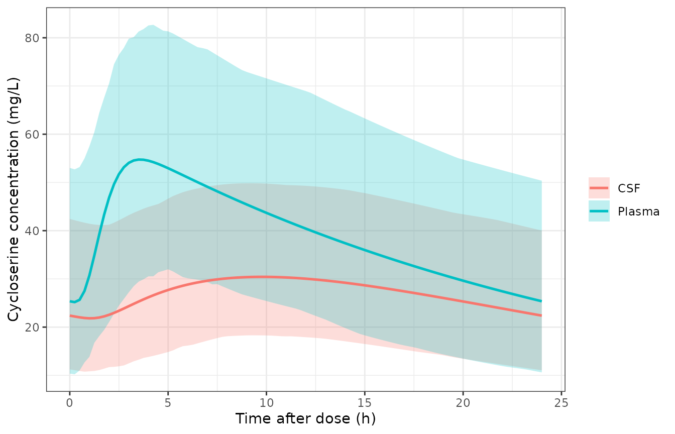
Replicates Figure 3A of Upton 2025: steady-state cycloserine in plasma and CSF after 750 mg terizidone once daily. Lines are the typical individual; ribbons the 5th-95th percentiles of 200 simulated participants.
The typical plasma peak of about 55 mg/L near 4 h and the CSF curve peaking near 30 mg/L around 10 h match Figure 3A (plasma peak about 53 mg/L, CSF about 30 mg/L).
PKNCA validation
conc_cyc <- sim_cyc |>
  dplyr::filter(!is.na(Cc)) |>
  dplyr::select(id, time, treatment, Plasma = Cc, CSF = Ccsf) |>
  tidyr::pivot_longer(c(Plasma, CSF), names_to = "matrix", values_to = "conc")
dose_cyc <- events_cyc |>
  dplyr::filter(evid == 1) |>
  dplyr::select(id, time, treatment, amt)

conc_obj <- PKNCA::PKNCAconc(conc_cyc, conc ~ time | treatment + id / matrix)
dose_obj <- PKNCA::PKNCAdose(dose_cyc, amt ~ time | treatment + id)
intervals <- data.frame(
  start = t_last, end = t_last + tau,
  cmax = TRUE, tmax = TRUE, auclast = TRUE
)
nca_cyc <- PKNCA::pk.nca(PKNCA::PKNCAdata(conc_obj, dose_obj, intervals = intervals))

sim_plasma <- as.data.frame(nca_cyc) |>
  dplyr::filter(matrix == "Plasma")

# Table S2 of Supplement S2: model-predicted plasma exposure for the study
# participants (geometric means), converted from ng/mL to mg/L.
ref_cyc <- data.frame(
  treatment = c("500 mg terizidone", "750 mg terizidone"),
  cmax = c(50.169, 52.687),
  tmax = c(3.6, 4.2),
  auclast = c(809.613, 844.225)
)
tbl_cyc <- ncaComparisonTable(
  sim_plasma, ref_cyc, by = "treatment",
  units = c(cmax = "mg/L", tmax = "h", auclast = "h*mg/L")
)
knitr::kable(tbl_cyc, caption = "Steady-state plasma cycloserine NCA: simulated median versus Table S2 geometric mean.")| NCA parameter | treatment | Reference | Simulated | % diff |
|---|---|---|---|---|
| Cmax (mg/L) | 500 mg terizidone | 50.2 | 35 | -30.3%* |
| Cmax (mg/L) | 750 mg terizidone | 52.7 | 51.8 | -1.8% |
| Tmax (h) | 500 mg terizidone | 3.6 | 3.75 | +4.2% |
| Tmax (h) | 750 mg terizidone | 4.2 | 4 | -4.8% |
| AUClast (h*mg/L) | 500 mg terizidone | 810 | 624 | -22.9%* |
| AUClast (h*mg/L) | 750 mg terizidone | 844 | 915 | +8.4% |
For the 750 mg arm (24 of the 27 participants) the simulated median Cmax, Tmax and AUC0-24 agree with the paper’s model-predicted values within about 10%. The 500 mg arm is starred: in the paper its three participants had almost the same exposure as the 750 mg arm (AUC0-24 810 versus 844 h*mg/L), which reflects those three individuals rather than the dose, whereas a virtual cohort drawn from the whole-study covariate distribution scales exposure with dose in the model’s linear kinetics.
# Medians of the 750 mg arm against Table S2. A mis-transcribed clearance,
# volume or dose conversion moves these by tens of percent.
med_750 <- sim_plasma |>
  dplyr::filter(treatment == "750 mg terizidone") |>
  dplyr::group_by(PPTESTCD) |>
  dplyr::summarise(median = median(PPORRES), .groups = "drop")
med_750 <- setNames(med_750$median, med_750$PPTESTCD)
stopifnot(
  abs(med_750[["cmax"]] / 52.687 - 1) < 0.2,
  abs(med_750[["auclast"]] / 844.225 - 1) < 0.2
)
CSF penetration
At steady state a linear effect compartment’s AUC over a dosing
interval is exactly ppc times the plasma AUC. The ratio is
computed per participant below; its median and the typical individual’s
value reproduce the published 69%.
ratio_cyc <- as.data.frame(nca_cyc) |>
  dplyr::filter(PPTESTCD == "auclast") |>
  dplyr::select(id, treatment, matrix, PPORRES) |>
  tidyr::pivot_wider(names_from = matrix, values_from = PPORRES) |>
  dplyr::mutate(ratio = CSF / Plasma)

auc_trap <- function(t, c) sum(diff(t) * (head(c, -1) + tail(c, -1)) / 2)
typ_ratio_cyc <- with(
  dplyr::filter(sim_cyc_typ, time >= t_last),
  auc_trap(time, Ccsf) / auc_trap(time, Cc)
)

ratio_cyc |>
  dplyr::group_by(treatment) |>
  dplyr::summarise(
    `Median CSF:plasma AUC0-24 ratio` = median(ratio),
    `Median plasma AUC0-24 (h*mg/L)` = median(Plasma),
    `Median CSF AUC0-24 (h*mg/L)` = median(CSF)
  ) |>
knitr::kable(digits = 3)| treatment | Median CSF:plasma AUC0-24 ratio | Median plasma AUC0-24 (h*mg/L) | Median CSF AUC0-24 (h*mg/L) |
|---|---|---|---|
| 500 mg terizidone | 0.694 | 624.204 | 434.267 |
| 750 mg terizidone | 0.689 | 914.954 | 632.319 |
Figure 2A of the paper shows individual model-derived medians of about 850 hmg/L (plasma) and 580 hmg/L (CSF) for AUC0-24, and about 48 mg/L and 27 mg/L for Cmax, consistent with the simulated cohort above.
Clofazimine
Figure 3B of the paper simulates 100 mg clofazimine once daily for 24 weeks. The same regimen is simulated here, with dense sampling on the last day of weeks 2, 8 and 24 for NCA. Because participants in the study had been treated for between 2 weeks and almost 2 years, their exposure spans these time points. With long-term daily dosing and only two occasion slots in the model, every dose is given occasion 1 here, so the between-occasion variability acts as additional between-subject variability.
n_dose_cfz <- 7 * 24
pk_days <- c(14, 56, 168)
obs_times <- sort(unique(c(
  seq(0, 24 * n_dose_cfz, by = 6),
  unlist(lapply(pk_days, function(d) seq(24 * (d - 1), 24 * d, by = 0.25)))
)))

make_cfz_events <- function(cohort) {
  dosing <- tidyr::expand_grid(id = cohort$id, time = 24 * (seq_len(n_dose_cfz) - 1)) |>
    dplyr::mutate(amt = 100, evid = 1L, cmt = "depot", dvid = NA_integer_)
  obs <- tidyr::expand_grid(id = cohort$id, time = obs_times) |>
    dplyr::mutate(amt = NA_real_, evid = 0L, cmt = "central", dvid = 1L)
  dplyr::bind_rows(dosing, obs) |>
    dplyr::left_join(cohort, by = "id") |>
    dplyr::mutate(OCC = 1, treatment = "100 mg clofazimine") |>
    dplyr::arrange(id, time, dplyr::desc(evid))
}

events_cfz <- make_cfz_events(cohort_cfz)
sim_cfz <- rxode2::rxSolve(
  mod_cfz, events = events_cfz, keep = c("treatment"), useLinCmt = FALSE
) |>
  as.data.frame()
#> ℹ parameter labels from comments will be replaced by 'label()'
#> Warning: some etas defaulted to non-mu referenced, possible parsing error: etaiov_fdepot_1, etaiov_fdepot_2, etaiov_mtt_1, etaiov_mtt_2, etaiov_ka_1, etaiov_ka_2
#> as a work-around try putting the mu-referenced expression on a simple line

sim_cfz_typ <- rxode2::rxSolve(
  rxode2::zeroRe(mod_cfz),
  events = make_cfz_events(tibble::tibble(id = 1L, WT = 52, FFM = 37.21, FM = 13.019)),
  useLinCmt = FALSE
) |>
  as.data.frame()
#> ℹ parameter labels from comments will be replaced by 'label()'
#> Warning: some etas defaulted to non-mu referenced, possible parsing error: etaiov_fdepot_1, etaiov_fdepot_2, etaiov_mtt_1, etaiov_mtt_2, etaiov_ka_1, etaiov_ka_2
#> as a work-around try putting the mu-referenced expression on a simple line
#> Warning: some etas defaulted to non-mu referenced, possible parsing error: etaiov_fdepot_1, etaiov_fdepot_2, etaiov_mtt_1, etaiov_mtt_2, etaiov_ka_1, etaiov_ka_2
#> as a work-around try putting the mu-referenced expression on a simple line
#> ℹ omega/sigma items treated as zero: 'etalcl', 'etalvc', 'etalvp', 'etalvp2', 'etalfdepot', 'etaiov_fdepot_1', 'etaiov_fdepot_2', 'etaiov_mtt_1', 'etaiov_mtt_2', 'etaiov_ka_1', 'etaiov_ka_2'
Replicating Figure 3B
grid_6h <- seq(0, 24 * n_dose_cfz, by = 6)
long_cfz <- sim_cfz |>
  dplyr::filter(time %in% grid_6h) |>
  tidyr::pivot_longer(c(Cc, Ccsf), names_to = "matrix", values_to = "conc") |>
  dplyr::mutate(matrix = ifelse(matrix == "Cc", "Plasma", "CSF")) |>
  dplyr::group_by(time, matrix) |>
  dplyr::summarise(lo = quantile(conc, 0.05), hi = quantile(conc, 0.95), .groups = "drop")
typ_cfz <- sim_cfz_typ |>
  dplyr::filter(time %in% grid_6h) |>
  tidyr::pivot_longer(c(Cc, Ccsf), names_to = "matrix", values_to = "conc") |>
  dplyr::mutate(matrix = ifelse(matrix == "Cc", "Plasma", "CSF"))

ggplot(dplyr::filter(long_cfz, time > 0), aes(time / (24 * 7), fill = matrix)) +
  geom_ribbon(aes(ymin = lo, ymax = hi), alpha = 0.25) +
  geom_line(data = dplyr::filter(typ_cfz, time > 0), aes(y = conc, colour = matrix)) +
  scale_y_log10() +
  labs(x = "Time (weeks)", y = "Clofazimine concentration (mg/L)",
       colour = NULL, fill = NULL) +
  theme_bw()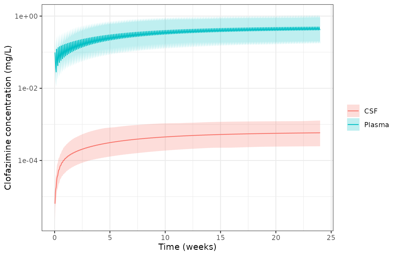
Replicates Figure 3B of Upton 2025: clofazimine in plasma and CSF over 24 weeks of 100 mg once daily. Lines are the typical individual; ribbons the 5th-95th percentiles of 200 simulated participants.
As in Figure 3B, typical plasma concentrations approach 0.5 mg/L by week 24 while CSF concentrations rise toward about 0.0006 mg/L.
PKNCA validation
conc_cfz <- sim_cfz |>
  dplyr::filter(!is.na(Cc)) |>
  dplyr::select(id, time, treatment, Plasma = Cc, CSF = Ccsf) |>
  tidyr::pivot_longer(c(Plasma, CSF), names_to = "matrix", values_to = "conc")
dose_cfz <- events_cfz |>
  dplyr::filter(evid == 1) |>
  dplyr::select(id, time, treatment, amt)

intervals_cfz <- data.frame(
  start = 24 * (pk_days - 1), end = 24 * pk_days,
  cmax = TRUE, tmax = TRUE, auclast = TRUE
)
nca_cfz <- PKNCA::pk.nca(PKNCA::PKNCAdata(
  PKNCA::PKNCAconc(conc_cfz, conc ~ time | treatment + id / matrix),
  PKNCA::PKNCAdose(dose_cfz, amt ~ time | treatment + id),
  intervals = intervals_cfz
))

cfz_summary <- as.data.frame(nca_cfz) |>
  dplyr::mutate(week = end / (24 * 7)) |>
  dplyr::group_by(matrix, week, PPTESTCD) |>
  dplyr::summarise(median = median(PPORRES), .groups = "drop") |>
  tidyr::pivot_wider(names_from = PPTESTCD, values_from = median)

cfz_summary |>
  dplyr::arrange(dplyr::desc(matrix), week) |>
  dplyr::select(matrix, week, cmax, tmax, auclast) |>
  dplyr::rename(
    Matrix = matrix, `Week of treatment` = week,
    `Cmax (mg/L)` = cmax, `Tmax (h)` = tmax, `AUC0-24 (h*mg/L)` = auclast
  ) |>
knitr::kable(digits = 5, caption = "Simulated median clofazimine NCA by duration of treatment.")| Matrix | Week of treatment | Cmax (mg/L) | Tmax (h) | AUC0-24 (h*mg/L) |
|---|---|---|---|---|
| Plasma | 2 | 0.22732 | 4.625 | 3.90453 |
| Plasma | 8 | 0.37355 | 4.625 | 7.57728 |
| Plasma | 24 | 0.50976 | 4.500 | 10.70911 |
| CSF | 2 | 0.00019 | 17.000 | 0.00445 |
| CSF | 8 | 0.00040 | 13.500 | 0.00963 |
| CSF | 24 | 0.00058 | 12.250 | 0.01389 |
plasma_wk <- dplyr::filter(cfz_summary, matrix == "Plasma")Table S1 reports a plasma geometric-mean Cmax of 0.486 mg/L, Tmax 5.0 h and AUC0-24 9.69 hmg/L across participants whose treatment duration ranged from 2 weeks to almost 2 years; Table S2’s model-predicted values are 0.502 mg/L, 5.5 h and 9.86 hmg/L. These fall between the simulated week-2 and week-24 medians, as expected for a drug still accumulating over months.
stopifnot(
  9.69 > plasma_wk$auclast[plasma_wk$week == 2],
  9.69 < 1.25 * plasma_wk$auclast[plasma_wk$week == 24],
  0.486 > plasma_wk$cmax[plasma_wk$week == 2],
  0.486 < 1.25 * plasma_wk$cmax[plasma_wk$week == 24]
)
CSF penetration
typ_last <- dplyr::filter(sim_cfz_typ, time >= 24 * 167, time <= 24 * 168)
typ_ratio_cfz <- auc_trap(typ_last$time, typ_last$Ccsf) / auc_trap(typ_last$time, typ_last$Cc)
typ_ratio_cfz
#> [1] 0.001296059
stopifnot(abs(typ_ratio_cfz / 0.0013 - 1) < 0.03)
After 24 weeks the CSF:plasma AUC ratio of the typical participant is within a few percent of the pseudo-partition coefficient of 0.0013 (0.13%); it sits just below it because plasma is still rising slowly and CSF lags plasma by an equilibration half-life of 55 h.
Assumptions and deviations
-
Cycloserine plasma additive error. The S1 control
stream builds the additive SD as
THETA(6) + 0.2 * LLOQwithLLOQ = 0.2mg/L hard-coded, and Table S3 prints the estimatedTHETA(6)(0.136 mg/L; its 95% CI starts at 0.0255, consistent with a bounded estimate rather than a total). The packagedaddSdis the total, 0.136 + 0.04 = 0.176 mg/L. The CSF additive terms, whoseTHETAis fixed at 0, are printed in Table S3 as totals and are used as printed. -
Cycloserine plasma estimates. Table S3 is used for
every structural value; the S1
$THETAblock agrees to rounding except for the age exponent (-0.0144 versus -0.0145) and proportional error (0.0762 versus 0.0760). The S1$OMEGAvariances reproduce the Table S3 percentages exactly as square roots and are used directly. -
Age centring. The equation centres age at 37 years
(
EXP(THETA(9)*(AGE-37))); the Results text calls it the cohort median and Table 1 prints 36. The equation is used. -
Clofazimine reference body sizes. Table S3 prints
the fixed Abdelwahab 2020 parameters re-expressed at the cohort’s
typical weight 52 kg, fat-free mass 37 kg and fat mass 13 kg (footnotes
d-f). The packaged model uses those printed values with the exact
reference values 52, 37.21 and 13.019 kg from the same paper’s control
stream (
TVWT,TVFFM,TVFAT). The allometric exponents and the parameter-to-covariate mapping come from the Abdelwahab 2020 control stream. One printed value is not exactly reproduced by that mapping: Vp2 = 889 L x (52/54) = 856 L with the published exponent of 1, whereas Table S3 prints 864 L (which 0.75 would give). The printed 864 L is used with the published exponent. - Clofazimine bioavailability. Abdelwahab 2020 includes a time-dependent rise in bioavailability over the first days of treatment (P-glycoprotein autoinhibition, half-life 1.44 days), applied only to its early bactericidal activity dataset. Upton 2025 Table S3 does not list it, and every Upton participant had been treated for at least 2 weeks, so the packaged model uses a constant relative bioavailability of 1.26. Simulations of the first days of treatment will therefore overstate early exposure slightly.
- Clofazimine variability. Table S3 prints the fixed Abdelwahab 2020 variabilities as percentages, described there as approximate %CV; they are converted as variance = (percentage / 100)^2, the convention Table S3 follows for cycloserine. Random effects that Abdelwahab 2020 declares but does not report (on Q1, Q2, ka, MTT between subjects, and on CL between occasions) are omitted.
-
Occasions. Both models carry two occasion slots
(
OCC = 1,2). Upton 2025 does not print its clofazimine plasma control stream, so the two-occasion structure for clofazimine follows the cycloserine model and the sampling design. -
A
non-mu referencednote is expected on model load. The occasion multiplexers (oc1 * etaiov_ka_1 + ...) place etas outside a mu-referenced position, so rxode2 emits “some etas defaulted to non-mu referenced”. This affects estimation efficiency, not simulation, and is shared by every IOV-multiplexing model in the library (for exampleAbdelgawad_2024_linezolid). - Figure 2B. The clofazimine CSF AUC0-24 and Cmax medians in Figure 2B (about 0.0017 h*mg/L and 0.00013 mg/L) are roughly seven-fold below what the published PPC of 0.0013 implies for the plasma medians shown beside them, and below the observed CSF range of 0.000127-0.00221 mg/L reported in the Results. Figure 3B and the stated 0.13% penetration agree with the packaged model; Figure 2B is not used for validation.
-
Dose units. Cycloserine doses are
cycloserine-equivalent mg. Convert terizidone with
2 * 102.09 / 302.28(750 mg terizidone = 506 mg cycloserine). - Concentrations are total drug. The pseudo-partition coefficients relate total CSF to total plasma concentrations, with no protein-binding correction.