Voriconazole and voriconazole N-oxide (Li 2021)
Source:vignettes/articles/Li_2021_voriconazole.Rmd
Li_2021_voriconazole.RmdModel and source
- Citation: Li S, Wu S, Gong W, Cao P, Chen X, Liu W, Xiang L, Wang Y, Huang J. Application of Population Pharmacokinetic Analysis to Characterize CYP2C19 Mediated Metabolic Mechanism of Voriconazole and Support Dose Optimization. Front Pharmacol. 2021;12:730826 (published 3 January 2022). doi:10.3389/fphar.2021.730826. PMCID PMC8762230.
- Description: Joint parent-metabolite population pharmacokinetic model for oral voriconazole and voriconazole N-oxide in Chinese immunocompromised patients with invasive fungal infection (Li 2021). Voriconazole: one compartment with first-order absorption (ka and F fixed) and parallel linear plus Michaelis-Menten elimination, where the Michaelis-Menten pathway forms the N-oxide and is inhibited by the N-oxide concentration through a fixed Imax/IC50 term. Voriconazole N-oxide: one compartment with first-order elimination. CYP2C19 metabolizer phenotype (IM, PM vs NM) acts exponentially on Vmax.
- Article: https://doi.org/10.3389/fphar.2021.730826 (open access)
- Supplement (Table S1, post-hoc exposures by CYP2C19 phenotype): https://www.frontiersin.org/articles/10.3389/fphar.2021.730826/full#supplementary-material
The article is volume 12 (2021) of Frontiers in Pharmacology; it was published online on 3 January 2022, which is why the journal’s own citation line reads “(2022)”. The model is named for the volume year, which is also the year in the DOI.
Population
Li 2021 analysed 427 plasma concentrations (214 voriconazole, 213 voriconazole N-oxide) from 78 immunocompromised patients treated with oral voriconazole 200 mg twice daily (no loading dose) for possible, probable or proven invasive fungal infection at Union Hospital, Wuhan, China, between February 2017 and July 2018 (Methods; Table 1). Patients were 14-70 years old (median 36.5; four adolescents aged 14-17) and weighed 44-111 kg (median 64); 57 were male and 21 female. Almost all samples were pre-dose troughs, taken 23-4,223 h after the first dose. Of the 75 genotyped patients, 27 were CYP2C19 normal metabolizers (NM, 1/1), 32 intermediate metabolizers (IM) and 16 poor metabolizers (PM); no *17 allele was found. Proton-pump inhibitors and glucocorticoids were recorded as co-medications but were not retained.
The same information is available programmatically via
readModelDb("Li_2021_voriconazole")()$population.
Source trace
Every ini() value carries an in-file comment pointing at
its source. The table below collects them. The equations come from Li
2021 Equations 8-13, which the maintainers read from the typeset article
(they did not survive text extraction of the PDF).
| Equation / parameter | Value | Source location |
|---|---|---|
lka (ka) |
fixed(log(1.1)) 1/h |
Table 2 ‘Ka 1.1 Fix’; Methods ‘Base Model’ (from Pascual 2012 / Wang 2014) |
lfdepot (F) |
fixed(log(0.895)) |
Table 2 ‘F 0.895 Fix’ |
lvc (V1) |
log(207.29) L |
Table 2 |
lcl (CL1) |
log(1.91) L/h |
Table 2 |
lvmax (Vmax, NM) |
log(18.80) mg/h |
Table 2 and footnote a |
lkm (km) |
fixed(log(1.15)) mg/L |
Table 2 ‘Km 1.15 Fix’; units from Results text below Table 2 |
imax (Imax) |
fixed(0.75) |
Table 2 ‘Imax 0.75 Fix’ |
lic50 (IC50) |
fixed(log(14.6)) mg/L |
Table 2 ‘IC50 14.6 Fix’ |
lvc_noxvori (V2) |
log(10.01) L |
Table 2 |
lcl_noxvori (CL2) |
log(4.65) L/h |
Table 2 |
e_cyp2c19_im_vmax |
-0.31 |
Table 2 ‘theta IM’; footnote a
Vmax = 18.80 * exp(theta_CYP2C19), theta_NM = 0 FIX |
e_cyp2c19_pm_vmax |
-0.61 |
Table 2 ‘theta PM’ |
etalvc |
2.4077^2 = 5.797 |
Table 2 ‘omega V1 (%) 240.77’ (omega = SD of eta; see below) |
etalcl |
0.0602^2 |
Table 2 ‘omega CL1 (%) 6.02’ |
etalcl_noxvori |
0.2557^2 |
Table 2 ‘omega CL2 (%) 25.57’ |
etalvmax |
0.2113^2 |
Table 2 ‘omega Vmax (%) 21.13’ |
propSd |
0.4697 |
Table 2 ‘VCZ-sigma (%) 46.97’ |
propSd_noxvori |
0.2793 |
Table 2 ‘VNO-sigma (%) 27.93’ |
d/dt(depot) |
-ka * depot |
Equation 8 |
d/dt(central) |
ka*depot - CL1/V1*A1 - CLnonlin/V1*A1 (F via
f(depot)) |
Equation 9 |
d/dt(central_noxvori) |
k_n*CLnonlin/V1*A1 - CL2/V2*A2 |
Equation 10 |
cl_nonlin |
Vmax/(C1 + km) * (1 - Imax*C2/(IC50 + C2)) |
Equation 11 |
Cc, Cc_noxvori
|
A1/V1, A2/V2
|
Equations 12-13 |
mw_ratio (k_n) |
365.31/349.31 = 1.0458 |
not printed; see Assumptions |
mod <- readModelDb("Li_2021_voriconazole")
ui <- rxode2::rxode(mod)
#> ℹ parameter labels from comments will be replaced by 'label()'
# The explicit ODEs must be integrated as written, not replaced by an
# automatic linear-compartment solution.
stopifnot(is.null(ui$linCmt))
om <- ui$omega
Structural self-checks
The Discussion states that Vmax “decreased by 26.7 and 45.7% in
patients with CYP2C19 IM and PM genotypes”. Those are exactly
1 - exp(theta) of the two Table 2 coefficients:
th <- ui$theta
red <- 100 * (1 - exp(th[c("e_cyp2c19_im_vmax", "e_cyp2c19_pm_vmax")]))
red
#> e_cyp2c19_im_vmax e_cyp2c19_pm_vmax
#>          26.65530          45.66491
stopifnot(abs(red - c(26.7, 45.7)) < 0.05)
Mass balance of Equation 10 at steady state: over one dosing
interval, the N-oxide eliminated (CL2 * AUC_VNO) must equal
k_n times the voriconazole that was not cleared by the
linear route (F * Dose - CL1 * AUC_VCZ). The check is on a
typical NM patient given 200 mg every 12 h for 60 days, so it exercises
the N-oxide feedback term at steady state.
ev_mb <- rbind(
  data.frame(time = seq(0, 1428, by = 12), evid = 1L, amt = 200, cmt = "depot", dvid = NA_integer_),
  data.frame(time = seq(1428, 1440, by = 0.05), evid = 0L, amt = NA, cmt = NA, dvid = 1L)
)
ev_mb <- ev_mb[order(ev_mb$time, -ev_mb$evid), ]
ev_mb$CYP2C19_IM <- 0L
ev_mb$CYP2C19_PM <- 0L
mb <- rxode2::rxSolve(
  rxode2::zeroRe(mod), ev_mb,
  returnType = "data.frame", rtol = 1e-10, atol = 1e-12, maxsteps = 1e6
)
#> ℹ parameter labels from comments will be replaced by 'label()'
#> ℹ omega/sigma items treated as zero: 'etalvc', 'etalcl', 'etalcl_noxvori', 'etalvmax'
trap <- function(t, y) sum(diff(t) * (head(y, -1) + tail(y, -1)) / 2)
auc_vcz <- trap(mb$time, mb$Cc)
auc_vno <- trap(mb$time, mb$Cc_noxvori)
lhs <- exp(th[["lcl_noxvori"]]) * auc_vno
rhs <- (365.31 / 349.31) * (0.895 * 200 - exp(th[["lcl"]]) * auc_vcz)
c(auc_vcz = auc_vcz, auc_vno = auc_vno, rel_diff = lhs / rhs - 1)
#>       auc_vcz       auc_vno      rel_diff
#>  2.547577e+01  2.931422e+01 -2.899868e-06
# Trapezoid on a 0.05 h grid over a slowly varying profile; measured ~1e-6.
stopifnot(abs(lhs / rhs - 1) < 1e-3)
Virtual cohort
The published Monte Carlo simulations (Table 3, Figure 6) drew 1,000 virtual patients per scenario. Here each phenotype arm has 196 virtual patients whose random effects are a Latin-hypercube design: every eta takes the 196 mid-point quantiles of its normal distribution exactly once (rescaled so the design reproduces the published variance), and the pairing across etas is a fixed permutation from R’s own generator. No random numbers are drawn by the simulation engine, so every number below is identical on any machine and any thread count, and the assertions can be tight. The same virtual patients are reused in every scenario, as in a common-random-numbers design.
n_sub <- 196L
q <- qnorm((seq_len(n_sub) - 0.5) / n_sub)
q <- q / sqrt(mean(q^2))
set.seed(20210730)
etas <- data.frame(
  etalvc = q * sqrt(om["etalvc", "etalvc"]),
  etalvmax = sample(q) * sqrt(om["etalvmax", "etalvmax"]),
  etalcl = sample(q) * sqrt(om["etalcl", "etalcl"]),
  etalcl_noxvori = sample(q) * sqrt(om["etalcl_noxvori", "etalcl_noxvori"])
)
# The design reproduces each published variance exactly.
design_var <- vapply(etas, function(x) mean(x^2), numeric(1))
stopifnot(max(abs(design_var / diag(om)[names(etas)] - 1)) < 1e-12)

pheno_levels <- c("NM", "IM", "PM")

# One arm: `ev` is a single-subject event table (doses and observations); it is
# replicated for every virtual patient, the patient's etas are attached as data
# columns, and the phenotype indicators are set.
make_arm <- function(ev, pheno, id_offset = 0L) {
  d <- ev[rep(seq_len(nrow(ev)), times = n_sub), ]
  d$id <- id_offset + rep(seq_len(n_sub), each = nrow(ev))
  d <- cbind(d, etas[rep(seq_len(n_sub), each = nrow(ev)), ])
  d$CYP2C19_IM <- as.integer(pheno == "IM")
  d$CYP2C19_PM <- as.integer(pheno == "PM")
  d$pheno <- pheno
  d
}

# Doses on `depot`; observations nominate the voriconazole endpoint through
# `dvid` (the model has two error endpoints, and both `Cc` and `Cc_noxvori`
# are returned as columns on every observation row).
dose_obs <- function(dose_times, amt, obs_times) {
  ev <- rbind(
    data.frame(time = dose_times, evid = 1L, amt = amt, cmt = "depot", dvid = NA_integer_),
    data.frame(time = obs_times, evid = 0L, amt = NA_real_, cmt = NA_character_, dvid = 1L)
  )
  ev[order(ev$time, -ev$evid), ]
}

solve_lhs <- function(events) {
  rxode2::rxSolve(
    mod, events,
    omega = NA, sigma = NA, keep = c("pheno", "regimen"),
    returnType = "data.frame", maxsteps = 1e6
  )
}
Replicate Table 3: trough attainment by regimen and phenotype
Table 3 lists, for 21 maintenance regimens, the median simulated voriconazole steady-state trough and the percentage of patients at or above 1, 2 and 5.5 mg/L. The paper does not say at which day the trough was read. Its Figure 6 simulations run for 20 days, and the published medians are reproduced by the trough at 480 h (day 20): reading the trough at 960 h raises every median by 10-16%, because patients with a large V1 are still accumulating at day 20. The comparison below uses the day-20 trough and, like the published medians, no residual error.
table3 <- tibble::tribble(
  ~pheno, ~dose, ~tau, ~pub_median, ~pub_ge1, ~pub_ge2, ~pub_ge5.5,
  "NM", 200, 12, 1.20, 56.09, 29.69, 2.48,
  "NM", 300, 12, 2.73, 78.36, 61.06, 19.78,
  "NM", 325, 12, 3.20, 81.05, 66.11, 25.76,
  "NM", 350, 12, 3.70, 83.59, 70.76, 32.00,
  "NM", 400, 12, 4.79, 86.91, 77.73, 43.66,
  "NM", 200, 8, 3.01, 82.27, 65.52, 22.59,
  "NM", 250, 8, 4.62, 88.69, 78.50, 41.84,
  "IM", 200, 12, 1.79, 69.08, 45.52, 6.12,
  "IM", 250, 12, 2.70, 79.58, 61.36, 17.50,
  "IM", 275, 12, 3.21, 82.74, 67.43, 23.95,
  "IM", 300, 12, 3.74, 85.21, 72.47, 30.81,
  "IM", 400, 12, 6.07, 90.36, 83.82, 54.67,
  "IM", 175, 8, 3.21, 84.95, 68.83, 23.32,
  "IM", 200, 8, 4.06, 88.35, 76.32, 34.34,
  "PM", 200, 12, 2.44, 78.83, 58.29, 11.99,
  "PM", 225, 12, 2.97, 82.81, 65.94, 19.30,
  "PM", 250, 12, 3.53, 85.56, 71.70, 26.56,
  "PM", 300, 12, 4.68, 89.14, 79.42, 41.36,
  "PM", 125, 8, 2.39, 80.20, 58.08, 10.56,
  "PM", 150, 8, 3.21, 86.04, 70.06, 21.63,
  "PM", 175, 8, 4.09, 89.56, 77.86, 34.00
) |>
  mutate(regimen = sprintf("%s %d mg q%dh", pheno, dose, tau))

t_trough <- 480
ev_t3 <- bind_rows(lapply(seq_len(nrow(table3)), function(i) {
  r <- table3[i, ]
  ev <- dose_obs(seq(0, t_trough - r$tau, by = r$tau), r$dose, t_trough)
  make_arm(ev, r$pheno, id_offset = (i - 1L) * n_sub) |>
    mutate(regimen = r$regimen)
}))
stopifnot(!anyDuplicated(unique(ev_t3[, c("id", "time", "evid")])))

sim_t3 <- solve_lhs(ev_t3) |> filter(time == t_trough)
#> ℹ parameter labels from comments will be replaced by 'label()'
stopifnot(nrow(sim_t3) == nrow(table3) * n_sub, !anyNA(sim_t3$Cc))

t3 <- sim_t3 |>
  group_by(regimen) |>
  summarise(
    sim_median = median(Cc),
    sim_ge1 = 100 * mean(Cc >= 1),
    sim_ge2 = 100 * mean(Cc >= 2),
    sim_ge5.5 = 100 * mean(Cc >= 5.5),
    .groups = "drop"
  ) |>
  inner_join(table3, by = "regimen") |>
  mutate(median_pct_diff = 100 * (sim_median / pub_median - 1)) |>
  arrange(match(pheno, pheno_levels), tau == 8, dose)
stopifnot(nrow(t3) == 21L)

t3 |>
  select(regimen, pub_median, sim_median, median_pct_diff,
         pub_ge1, sim_ge1, pub_ge2, sim_ge2, pub_ge5.5, sim_ge5.5) |>
  rename(
    "Regimen" = regimen,
    "Median (paper, mg/L)" = pub_median,
    "Median (sim, mg/L)" = sim_median,
    "Median % diff" = median_pct_diff,
    ">=1 paper (%)" = pub_ge1, ">=1 sim (%)" = sim_ge1,
    ">=2 paper (%)" = pub_ge2, ">=2 sim (%)" = sim_ge2,
    ">=5.5 paper (%)" = pub_ge5.5, ">=5.5 sim (%)" = sim_ge5.5
  ) |>
knitr::kable(digits = 2, caption = "Replicates Table 3 of Li 2021 (day-20 trough).")| Regimen | Median (paper, mg/L) | Median (sim, mg/L) | Median % diff | >=1 paper (%) | >=1 sim (%) | >=2 paper (%) | >=2 sim (%) | >=5.5 paper (%) | >=5.5 sim (%) |
|---|---|---|---|---|---|---|---|---|---|
| NM 200 mg q12h | 1.20 | 1.21 | 0.94 | 56.09 | 58.16 | 29.69 | 12.76 | 2.48 | 0.00 |
| NM 300 mg q12h | 2.73 | 2.71 | -0.67 | 78.36 | 75.00 | 61.06 | 61.73 | 19.78 | 2.04 |
| NM 325 mg q12h | 3.20 | 3.22 | 0.72 | 81.05 | 75.51 | 66.11 | 66.84 | 25.76 | 8.67 |
| NM 350 mg q12h | 3.70 | 3.66 | -0.99 | 83.59 | 78.06 | 70.76 | 69.90 | 32.00 | 21.43 |
| NM 400 mg q12h | 4.79 | 4.55 | -5.08 | 86.91 | 80.61 | 77.73 | 73.47 | 43.66 | 41.84 |
| NM 200 mg q8h | 3.01 | 3.01 | 0.15 | 82.27 | 78.57 | 65.52 | 67.35 | 22.59 | 3.57 |
| NM 250 mg q8h | 4.62 | 4.74 | 2.62 | 88.69 | 83.67 | 78.50 | 77.04 | 41.84 | 39.29 |
| IM 200 mg q12h | 1.79 | 1.74 | -3.06 | 69.08 | 68.88 | 45.52 | 43.37 | 6.12 | 0.00 |
| IM 250 mg q12h | 2.70 | 2.68 | -0.91 | 79.58 | 75.00 | 61.36 | 61.22 | 17.50 | 1.53 |
| IM 275 mg q12h | 3.21 | 3.10 | -3.36 | 82.74 | 77.55 | 67.43 | 67.86 | 23.95 | 4.59 |
| IM 300 mg q12h | 3.74 | 3.58 | -4.39 | 85.21 | 78.57 | 72.47 | 69.90 | 30.81 | 18.88 |
| IM 400 mg q12h | 6.07 | 5.99 | -1.25 | 90.36 | 83.16 | 83.82 | 77.04 | 54.67 | 55.10 |
| IM 175 mg q8h | 3.21 | 3.23 | 0.70 | 84.95 | 81.12 | 68.83 | 70.41 | 23.32 | 4.08 |
| IM 200 mg q8h | 4.06 | 4.15 | 2.13 | 88.35 | 82.65 | 76.32 | 75.00 | 34.34 | 25.51 |
| PM 200 mg q12h | 2.44 | 2.35 | -3.76 | 78.83 | 73.98 | 58.29 | 58.16 | 11.99 | 0.00 |
| PM 225 mg q12h | 2.97 | 2.83 | -4.79 | 82.81 | 77.04 | 65.94 | 64.29 | 19.30 | 1.53 |
| PM 250 mg q12h | 3.53 | 3.41 | -3.29 | 85.56 | 79.08 | 71.70 | 68.37 | 26.56 | 8.16 |
| PM 300 mg q12h | 4.68 | 4.58 | -2.04 | 89.14 | 81.12 | 79.42 | 73.98 | 41.36 | 37.76 |
| PM 125 mg q8h | 2.39 | 2.36 | -1.22 | 80.20 | 77.55 | 58.08 | 59.18 | 10.56 | 0.00 |
| PM 150 mg q8h | 3.21 | 3.26 | 1.43 | 86.04 | 81.12 | 70.06 | 68.37 | 21.63 | 1.53 |
| PM 175 mg q8h | 4.09 | 4.22 | 3.06 | 89.56 | 83.67 | 77.86 | 74.49 | 34.00 | 21.43 |
The medians are the load-bearing check: a mis-transcribed Vmax, CL1, F, CYP2C19 coefficient or IIV scale moves them by tens of percent. The design is deterministic, so the bounds are set from the achieved values (median difference -1.0%, median |difference| 2.0%, largest |difference| 5.1%). The 1 and 2 mg/L attainment percentages are reproduced to within about 8 percentage points, except for the NM 200 mg q12h row at 2 mg/L (see Assumptions and deviations), which is excluded from that gate.
ge2_rows <- t3$regimen != "NM 200 mg q12h"
stopifnot(
  abs(median(t3$median_pct_diff)) < 3,
  max(abs(t3$median_pct_diff)) < 7,
  max(abs(t3$sim_ge1 - t3$pub_ge1)) < 10,
  max(abs(t3$sim_ge2 - t3$pub_ge2)[ge2_rows]) < 8
)
Why Table 2’s omega is an SD
Table 2 reports the between-subject variability as “omega (%)” and
its footnote defines omega as the “square root of interindividual
variance”, so the model uses (omega / 100)^2 as the
variance. For the V1 value of 240.77% this matters: read as a
coefficient of variation instead, the variance would be
log(1 + 2.4077^2) = 1.92 rather than 5.80. The Table 3
medians adjudicate between the two readings, because a smaller V1 spread
raises the median trough at day 20:
cv_var <- log(1 + 2.4077^2)
etas_cv <- etas
etas_cv$etalvc <- q * sqrt(cv_var)
adj_rows <- c("NM 200 mg q12h", "NM 400 mg q12h", "IM 200 mg q12h", "PM 200 mg q12h", "PM 150 mg q8h")
ev_cv <- ev_t3 |>
  filter(regimen %in% adj_rows) |>
  mutate(etalvc = etas_cv$etalvc[((id - 1L) %% n_sub) + 1L])
cv_tab <- solve_lhs(ev_cv) |>
  filter(time == t_trough) |>
  group_by(regimen) |>
  summarise(median_cv_reading = median(Cc), .groups = "drop") |>
  inner_join(t3 |> select(regimen, pub_median, sim_median), by = "regimen") |>
  mutate(
    pct_sd_reading = 100 * (sim_median / pub_median - 1),
    pct_cv_reading = 100 * (median_cv_reading / pub_median - 1)
  )
cv_tab |>
  rename(
    "Regimen" = regimen, "Paper median" = pub_median,
    "SD reading" = sim_median, "CV reading" = median_cv_reading,
    "SD reading % diff" = pct_sd_reading, "CV reading % diff" = pct_cv_reading
  ) |>
knitr::kable(digits = 2, caption = "Median day-20 trough under the two readings of 'omega V1 (%) 240.77'.")| Regimen | CV reading | Paper median | SD reading | SD reading % diff | CV reading % diff |
|---|---|---|---|---|---|
| IM 200 mg q12h | 2.32 | 1.79 | 1.74 | -3.06 | 29.75 |
| NM 200 mg q12h | 1.58 | 1.20 | 1.21 | 0.94 | 31.51 |
| NM 400 mg q12h | 6.27 | 4.79 | 4.55 | -5.08 | 31.00 |
| PM 150 mg q8h | 4.01 | 3.21 | 3.26 | 1.43 | 25.06 |
| PM 200 mg q12h | 3.12 | 2.44 | 2.35 | -3.76 | 27.97 |
Replicate Figure 6: the standard regimen over 20 days
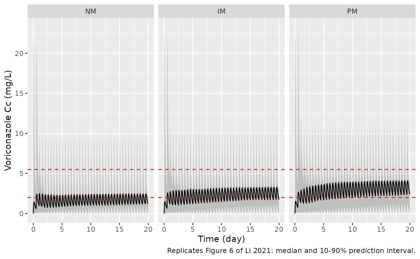
Figure 6 shows the simulated voriconazole profile over the first 20 days of the standard regimen (400 mg every 12 h for two doses, then 200 mg every 12 h) for each phenotype, as a median and a 10-90% band. The Results state that the steady-state troughs reach the 2-5.5 mg/L range in PMs while those of IMs and NMs stay below it.
fig6_times <- sort(unique(c(seq(0, 480, by = 1), seq(12, 480, by = 12))))
fig6_doses <- seq(0, 468, by = 12)
fig6_amt <- ifelse(fig6_doses < 24, 400, 200)
ev_f6 <- bind_rows(lapply(seq_along(pheno_levels), function(i) {
  make_arm(dose_obs(fig6_doses, fig6_amt, fig6_times), pheno_levels[i], id_offset = (i - 1L) * n_sub) |>
    mutate(regimen = "standard")
}))
sim_f6 <- solve_lhs(ev_f6) |>
  mutate(pheno = factor(pheno, levels = pheno_levels))
stopifnot(!anyNA(sim_f6$Cc))

sim_f6 |>
  group_by(pheno, time) |>
  summarise(
    lo = quantile(Cc, 0.1), med = median(Cc), hi = quantile(Cc, 0.9),
    .groups = "drop"
  ) |>
  ggplot(aes(time / 24, med)) +
  geom_ribbon(aes(ymin = lo, ymax = hi), fill = "grey75") +
  geom_line() +
  geom_hline(yintercept = c(2, 5.5), linetype = "dashed", colour = "firebrick") +
  facet_wrap(~pheno, nrow = 1) +
  labs(
    x = "Time (day)", y = "Voriconazole Cc (mg/L)",
    caption = "Replicates Figure 6 of Li 2021: median and 10-90% prediction interval."
  )
trough_d20 <- sim_f6 |>
  filter(time == 480) |>
  group_by(pheno) |>
  summarise(median_trough = median(Cc), .groups = "drop")
knitr::kable(trough_d20, digits = 2, caption = "Median day-20 trough, standard regimen.")| pheno | median_trough |
|---|---|
| NM | 1.24 |
| IM | 1.74 |
| PM | 2.42 |
# Deterministic design; realised 1.24 / 1.74 / 2.42 mg/L.
stopifnot(
  trough_d20$median_trough[trough_d20$pheno == "NM"] < 2,
  trough_d20$median_trough[trough_d20$pheno == "IM"] < 2,
  trough_d20$median_trough[trough_d20$pheno == "PM"] > 2,
  trough_d20$median_trough[trough_d20$pheno == "PM"] < 5.5
)
PKNCA: day-7 exposure of voriconazole and its N-oxide
Supplementary Table S1 reports the day-7 steady-state exposure of both analytes (AUC over 144-168 h, Cmax and Cmin, mean (SD)) per phenotype for 200 mg every 12 h without a loading dose, the regimen the patients actually received. Those values are post-hoc (empirical Bayes) predictions for the 74 genotyped study patients, not a population simulation, so they are expected to agree only approximately with the virtual cohort: the study data were almost all troughs, so the individual V1 estimates shrink toward the typical value, and the post-hoc Cmax is correspondingly less extreme than a simulated one whose V1 spread is the full published omega.
obs_d7 <- seq(144, 168, by = 0.25)
ev_d7 <- bind_rows(lapply(seq_along(pheno_levels), function(i) {
  make_arm(dose_obs(seq(0, 156, by = 12), 200, obs_d7), pheno_levels[i], id_offset = (i - 1L) * n_sub) |>
    mutate(regimen = "200 mg q12h")
}))
sim_d7 <- solve_lhs(ev_d7)
stopifnot(!anyNA(sim_d7$Cc), !anyNA(sim_d7$Cc_noxvori))

dose_d7 <- ev_d7 |>
  filter(evid == 1) |>
  select(id, time, amt, pheno)

nca_one <- function(conc_col) {
  conc <- sim_d7 |>
    filter(!is.na(.data[[conc_col]])) |>
    transmute(id, time, pheno, conc = .data[[conc_col]])
  conc_obj <- PKNCA::PKNCAconc(conc, conc ~ time | pheno + id)
  dose_obj <- PKNCA::PKNCAdose(dose_d7, amt ~ time | pheno + id)
  intervals <- data.frame(start = 144, end = 168, auclast = TRUE, cmax = TRUE, cmin = TRUE)
  PKNCA::pk.nca(PKNCA::PKNCAdata(conc_obj, dose_obj, intervals = intervals))
}
nca_vcz <- nca_one("Cc")
nca_vno <- nca_one("Cc_noxvori")

# Table S1 reports means; aggregate the simulated per-subject values the same way.
mean_wide <- function(res) {
  as.data.frame(res) |>
    filter(PPTESTCD %in% c("auclast", "cmax", "cmin")) |>
    group_by(pheno, PPTESTCD) |>
    summarise(value = mean(PPORRES), .groups = "drop") |>
    pivot_wider(names_from = PPTESTCD, values_from = value)
}
sim_vcz <- mean_wide(nca_vcz)
sim_vno <- mean_wide(nca_vno)

s1_vcz <- tibble::tribble(
  ~pheno, ~cmin, ~cmax, ~auclast,
  "NM", 1.34, 2.83, 51.37,
  "IM", 1.99, 3.06, 62.18,
  "PM", 2.84, 4.30, 88.10
)
s1_vno <- tibble::tribble(
  ~pheno, ~cmin, ~cmax, ~auclast,
  "NM", 2.22, 2.49, 57.46,
  "IM", 2.01, 2.19, 51.09,
  "PM", 2.51, 2.64, 62.14
)
nca_units <- c(cmin = "mg/L", cmax = "mg/L", auclast = "mg*h/L")

cmp_vcz <- nlmixr2lib::ncaComparisonTable(
  simulated = sim_vcz, reference = s1_vcz, by = "pheno",
  units = nca_units, tolerance_pct = 20
)
knitr::kable(cmp_vcz, caption = "Voriconazole, day 7 (144-168 h): simulated mean vs Table S1 mean. * differs by >20%.")| NCA parameter | pheno | Reference | Simulated | % diff |
|---|---|---|---|---|
| Cmax (mg/L) | NM | 2.83 | 4.76 | +68.1%* |
| Cmax (mg/L) | IM | 3.06 | 5.29 | +73.0%* |
| Cmax (mg/L) | PM | 4.3 | 5.79 | +34.7%* |
| Cmin (mg/L) | NM | 1.34 | 0.869 | -35.1%* |
| Cmin (mg/L) | IM | 1.99 | 1.24 | -37.5%* |
| Cmin (mg/L) | PM | 2.84 | 1.63 | -42.7%* |
| AUClast (mg*h/L) | NM | 51.4 | 47.3 | -8.0% |
| AUClast (mg*h/L) | IM | 62.2 | 59.1 | -5.0% |
| AUClast (mg*h/L) | PM | 88.1 | 70.4 | -20.1%* |
cmp_vno <- nlmixr2lib::ncaComparisonTable(
  simulated = sim_vno, reference = s1_vno, by = "pheno",
  units = nca_units, tolerance_pct = 20
)
knitr::kable(cmp_vno, caption = "Voriconazole N-oxide, day 7 (144-168 h): simulated mean vs Table S1 mean. * differs by >20%.")| NCA parameter | pheno | Reference | Simulated | % diff |
|---|---|---|---|---|
| Cmax (mg/L) | NM | 2.49 | 2.25 | -9.5% |
| Cmax (mg/L) | IM | 2.19 | 1.81 | -17.4% |
| Cmax (mg/L) | PM | 2.64 | 1.43 | -45.8%* |
| Cmin (mg/L) | NM | 2.22 | 1.57 | -29.3%* |
| Cmin (mg/L) | IM | 2.01 | 1.37 | -31.8%* |
| Cmin (mg/L) | PM | 2.51 | 1.14 | -54.4%* |
| AUClast (mg*h/L) | NM | 57.5 | 47 | -18.2% |
| AUClast (mg*h/L) | IM | 51.1 | 39 | -23.7%* |
| AUClast (mg*h/L) | PM | 62.1 | 31.5 | -49.4%* |
The voriconazole AUC, the quantity the paper uses to show the CYP2C19 effect, agrees within about 20% in every phenotype and preserves the NM < IM < PM ordering (Table S1: p = 0.005 for PM vs IM and < 0.001 for PM vs NM). That is gated:
auc_cmp <- inner_join(
  sim_vcz |> select(pheno, sim = auclast),
  s1_vcz |> select(pheno, pub = auclast),
  by = "pheno"
) |>
  mutate(pct = 100 * (sim / pub - 1))
auc_cmp
#> # A tibble: 3 × 4
#>   pheno   sim   pub    pct
#>   <chr> <dbl> <dbl>  <dbl>
#> 1 IM     59.1  62.2  -5.03
#> 2 NM     47.3  51.4  -7.98
#> 3 PM     70.4  88.1 -20.1
# Deterministic design; realised -8.0 / -5.0 / -20.1 %.
stopifnot(
  nrow(auc_cmp) == 3L,
  max(abs(auc_cmp$pct)) < 22,
  sim_vcz$auclast[sim_vcz$pheno == "NM"] < sim_vcz$auclast[sim_vcz$pheno == "IM"],
  sim_vcz$auclast[sim_vcz$pheno == "IM"] < sim_vcz$auclast[sim_vcz$pheno == "PM"]
)
The remaining rows are shown for completeness and are not gated. The simulated mean Cmax is higher and the mean Cmin lower than the post-hoc values, as expected from the shrinkage of the post-hoc V1 described above. The simulated N-oxide exposure falls from NM to PM because the model routes the N-oxide formation through the CYP2C19-dependent Vmax, while the post-hoc N-oxide exposures in Table S1 do not differ between phenotypes (p > 0.2), a point the Discussion attributes to other enzymes contributing to N-oxidation. The published model has no such second formation route, so the population simulation cannot reproduce that flat pattern; in the fitted data the individual CL2 estimates absorb it.
Assumptions and deviations
-
The factor
k_nin Equation 10 is not given. Equation 10 multiplies the N-oxide formation flux byk_n, which is neither defined nor valued in the article or its supplement and is not one of the 11 (base) / 13 (final) estimated parameters. The Results define the N-oxide input rate as “the same as the conversion rate from VCZ to VNO”, and both analytes are measured in mg/L, so the maintainers tookk_nas the stoichiometric molar-mass ratio 365.31 / 349.31 = 1.0458 (voriconazole C16H14F3N5O plus one oxygen). If the authors instead usedk_n = 1, N-oxide concentrations would be 4.4% lower and voriconazole concentrations essentially unchanged (only through the N-oxide inhibition term). - IIV scale. Table 2’s “omega (%)” is read as 100 times the SD of eta, as the table footnote defines it; the CV reading is rejected by Table 3 (see “Why Table 2’s omega is an SD”). The V1 variance is therefore 5.80, which spans V1 from about 2 L to over 20,000 L between the 2.5th and 97.5th percentiles. That spread is as published and reflects that V1 was estimated from trough data only (Discussion, limitations).
- Day of the Table 3 trough. The article does not state when the simulated “steady-state” trough was read. The day-20 trough (the Figure 6 horizon) reproduces the published medians; later days do not, because patients with a large V1 are far from steady state at day 20.
- Attainment tails not reproduced. The simulated share of troughs at or above 5.5 mg/L is below the published value in every regimen whose median trough is under about 3.5 mg/L (for 200 mg q12h it is 0% in every phenotype, against 2.48%, 6.12% and 11.99% published), and the NM 200 mg q12h share at or above 2 mg/L is 13% against 29.69%. The published medians are reproduced, so the published Monte Carlo distribution has a wider upper tail than the Table 2 between-subject variability alone produces. Adding the 47% proportional residual error widens the tail but lowers the median by about 20%, so no single reading reproduces all four columns; the article does not describe how its percentages were computed. These cells are shown in the Table 3 comparison but excluded from its gate.
- Units of km. Table 2 prints km without a unit; the Results text below it states that “km, Imax, and IC50 were fixed at 1.15 mg/L, 0.75 and 14.6 mg/L”, so km is in mg/L like both concentrations.
-
Bioavailability. Equation 9 applies F to the
absorption flux (
F * Agut * ka); the model applies it to the dose throughf(depot), which is equivalent for a first-order depot. - Virtual cohort. Only the CYP2C19 phenotype enters the model, so no other covariates are simulated. Each phenotype arm is simulated separately, as in the article.
- Errata. No correction notice for this article was found on the journal’s page or on PubMed as of 2026-09-30.