Dioxin-like compound mixture PBPK (Liu 2022)
Source:vignettes/articles/Liu_2022_dioxin_mixture_pbpk.Rmd
Liu_2022_dioxin_mixture_pbpk.RmdModel and source
Liu, Zacharewski, Conolly and Zhang (2022, Toxics 10(11):700, doi:10.3390/toxics10110700) present a physiologically based pharmacokinetic (PBPK) modeling framework for mixtures of dioxin-like compounds (DLCs) in humans. DLCs (polychlorinated dibenzo-p-dioxins, dibenzofurans and biphenyls, with 2,3,7,8-TCDD as the reference congener) are persistent lipophilic pollutants taken up chronically through the diet. Their toxicokinetics are nonlinear: in the liver each congener binds reversibly to the aryl hydrocarbon receptor (AHR) and to CYP1A2, and the AHR-liganded congener induces CYP1A2, which both sequesters and metabolises the congeners. In a mixture, congeners therefore compete for AHR and CYP1A2 and cross-induce CYP1A2 - an interaction that cannot be captured by simulating each congener alone.
The framework adapts the human TCDD model of Emond et al. Blood is a quasi-steady-state algebraic compartment; fat, rest-of-body and liver are each split into a blood subcompartment and a diffusion-limited tissue subcompartment. Liver tissue carries the AHR / CYP1A2 binding and the CYP1A2 mRNA -> protein induction cascade. Body weight and all tissue volume / flow fractions are polynomial functions of age, so each run is a lifetime (0-70 year) forward simulation of constant daily dietary intake - there are no dose records and the model is deterministic.
The authors implemented the model in GNU Octave and published the
full source (parameters, ODEs and the chemical-specific parameter
spreadsheet) at https://github.com/pulsatility/2022-DLC-Mixture-PBPK,
which the paper (Section 2.6) designates as the model source. The
parameter values and equations used here are transcribed from that code
(DLC_human_cmd.m, DLC_human_ode.m,
DLC_human_parameters.xlsx; paper Tables S1-S3).
Two instances of the framework are shipped:
-
Liu_2022_tcdd_pbpk- the single-congener (TCDD) model, the framework’s validation case (paper Figure 2, which reproduces the Emond model exactly). -
Liu_2022_dioxin_mixture_pbpk- a binary TCDD + 2,3,4,7,8-PeCDF mixture, demonstrating the cross-induction result (paper Figure 3A).
tcdd <- rxode2::rxode2(readModelDb("Liu_2022_tcdd_pbpk"))
mix <- rxode2::rxode2(readModelDb("Liu_2022_dioxin_mixture_pbpk"))- Citation: Liu R, Zacharewski TR, Conolly RB, Zhang Q. A Physiologically Based Pharmacokinetic (PBPK) Modeling Framework for Mixtures of Dioxin-like Compounds. Toxics. 2022;10(11):700. doi:10.3390/toxics10110700. Physiological and biochemical parameters from the authors’ Octave code DLC_human_cmd.m / DLC_human_ode.m and chemical-specific TCDD parameters from DLC_human_parameters.xlsx (https://github.com/pulsatility/2022-DLC-Mixture-PBPK; paper Tables S1-S3). Structural parent model: Emond C et al. Environ Health Perspect 2005;113(12):1666-1668 and Toxicol Sci 2004;80(1):115-133.
Population
This is a mechanistic forward-simulation model, not a fit to a
clinical cohort. The physiology is the Emond human model (tissue volumes
and blood flows as polynomial functions of age; Wang et al. 1997), run
for a female from birth to 70 years. Exposure is a constant daily
dietary intake per congener, driven at the EPA reference dose (RfD,
0.0007 ng/kg bw/day) and point-of-departure dose (PoD, 0.02 ng/kg
bw/day) lifetime scenarios. The paper’s population Monte Carlo analysis
(its Figure 5) samples total AHR, CYP1A2 transcription / basal levels,
CYP1A2 Emax, the body-weight polynomial and the dietary intake of 11
congeners; those distributions are summarised in the model
population metadata but are not encoded as random effects
here (the model is deterministic).
readModelDb("Liu_2022_tcdd_pbpk")()$population[c("species", "age_range", "dose_range")]
#> $species
#> [1] "human"
#>
#> $age_range
#> [1] "0-70 years (lifetime forward simulation)"
#>
#> $dose_range
#> [1] "Constant daily dietary intake. The paper runs an EPA reference dose (RfD, 0.0007 ng/kg bw/day) and point-of-departure dose (PoD, 0.02 ng/kg bw/day) lifetime scenario; MSTOT defaults to the PoD dose."
Source trace
Every ini() parameter carries an in-file comment
pointing to its origin in the authors’ Octave code / parameter
spreadsheet. Key structural choices:
| Equation / parameter | Value | Source location |
|---|---|---|
| Blood (quasi-steady state, algebraic) | - |
DLC_human_ode.m CB
|
| Diffusion-limited fat / RB / liver tissue | - |
DLC_human_ode.m ODEs 5-10 |
AHR binding Kd,AHR (TCDD) |
0.1 nM |
DLC_human_parameters.xlsx KDAHR
|
kb,AHR |
6 /h | paper Section 2.3 (“we set it to 6/h”) |
CYP1A2 binding Kd,1A2
|
40 nM |
xlsx KD1A2
|
| CYP1A2 induction Emax / EC50 / Hill | 9300 / 130 nM / 0.6 |
DLC_human_cmd.m, DLC_human_ode.m
|
| CYP1A2 basal (initial) | 1600 nM |
DLC_human_cmd.m CYP1A2_1BASAL
|
Hepatic elimination kelim (TCDD) |
0.0011 /h |
xlsx kelim
|
Partition coefficients
PL/PF/PRB (TCDD) |
6 / 100 / 1.5 | xlsx |
| Growth / volume polynomials (female) | - | DLC_human_ode.m |
Validation against the authors’ reference implementation
The strongest available check is reproduction of the authors’ own
Octave model. Running DLC_human_ode.m (verbatim) for the
single-TCDD and the binary TCDD + PeCDF cases yields the tissue
concentrations below at the eight ages the paper scatter-plots in Figure
2B. The packaged rxode2 models must reproduce these to integrator
tolerance (the two implementations share identical parameters, so any
difference is pure numerical error).
# Reference output of the authors' Octave code (DLC_human_ode.m), female.
# Columns: year, CA, CF, CRB, CL (total liver), CYP1A2 (free, nM).
ref_tcdd_high <- as.data.frame(do.call(rbind, list(
  c(1, 0.0004752823385, 0.04585359264, 0.0007124136162, 0.2261675182, 18730.81163),
  c(10, 0.001683453231, 0.1669597553, 0.002524947414, 1.609063533, 37940.59732),
  c(20, 0.002019160798, 0.2002846614, 0.003028699096, 2.136984426, 42044.22034),
  c(30, 0.002282740832, 0.2273015476, 0.003424082144, 2.58723345, 45055.86035),
  c(40, 0.002532412987, 0.253053741, 0.003798593922, 3.04158104, 47771.19626),
  c(50, 0.002693638141, 0.2696631966, 0.004040442755, 3.34889642, 49462.93963),
  c(60, 0.002725673327, 0.2728344271, 0.004088514447, 3.411510536, 49795.40668),
  c(70, 0.002615174887, 0.2612254096, 0.003922785398, 3.198696246, 48649.61923)
)))
names(ref_tcdd_high) <- c("year", "CA", "CF", "CRB", "CL", "CYP")

ref_tcdd_low <- as.data.frame(do.call(rbind, list(
  c(1, 2.859622848e-05, 0.002752792668, 4.286141748e-05, 0.003692457412, 4789.488696),
  c(10, 0.0001375501738, 0.01363323401, 0.0002063040658, 0.03493473979, 9784.584703),
  c(20, 0.00017018765, 0.01687623487, 0.0002552772614, 0.04796207462, 10898.09831),
  c(30, 0.0002051219412, 0.02039887323, 0.0003076780594, 0.063434271, 11996.81454),
  c(40, 0.0002531608954, 0.02525558411, 0.0003797354479, 0.08710258389, 13390.92554),
  c(50, 0.0003004094215, 0.03003377966, 0.0004506089893, 0.1128851484, 14660.81984),
  c(60, 0.0003275725556, 0.03277036245, 0.0004913575589, 0.1287697037, 15354.46011),
  c(70, 0.0003161010399, 0.0315891858, 0.0004741557633, 0.1219833922, 15065.2614)
)))
names(ref_tcdd_low) <- c("year", "CA", "CF", "CRB", "CL", "CYP")

# Binary TCDD + PeCDF, each at PoD (0.02 ng/kg/day).
# Columns: year, TCDD[CA CF CRB CL], PeCDF[CA CF CRB CL], CYP1A2.
ref_bin <- as.data.frame(do.call(rbind, list(
  c(1, 0.00042756585, 0.0412646, 0.00064089545, 0.24297473, 0.00034990559, 0.045288913, 0.0011063204, 0.20597163, 22460.876),
  c(10, 0.001435269, 0.14236774, 0.002152711, 1.6745916, 0.0014517792, 0.19510039, 0.0045962913, 1.7244181, 46422.124),
  c(20, 0.00169754, 0.16840313, 0.0025462772, 2.2252945, 0.0018897718, 0.2540512, 0.00598404, 2.5177863, 52195.479),
  c(30, 0.0018866034, 0.18791254, 0.0028298856, 2.668139, 0.0022526962, 0.30434759, 0.0071333451, 3.2345621, 56347.02),
  c(40, 0.0020432841, 0.20425191, 0.0030649115, 3.0838711, 0.0026468183, 0.35926375, 0.0083813915, 4.0523659, 60162.82),
  c(50, 0.0021213545, 0.21243485, 0.0031820259, 3.3405127, 0.0029818266, 0.4058321, 0.0094422953, 4.7607909, 62788.987),
  c(60, 0.0021115052, 0.21138364, 0.0031672638, 3.3716316, 0.003151567, 0.42905952, 0.0099799323, 5.1017177, 63672.551),
  c(70, 0.0020252708, 0.20227637, 0.0030379217, 3.1712343, 0.0030607917, 0.41579757, 0.0096926411, 4.8601557, 62426.629)
)))
names(ref_bin) <- c("year", "CA1", "CF1", "CRB1", "CL1", "CA2", "CF2", "CRB2", "CL2", "CYP")
# Forward lifetime solve on a half-yearly grid (hours). Tight tolerances so the
# comparison against the reference implementation reflects the model, not the
# integrator.
tgrid <- seq(0, 24 * 365 * 70, by = 24 * 365 / 2)
ev <- rxode2::et(tgrid)

solve_tcdd <- function(mod, mstot) {
  s <- rxode2::rxSolve(mod, ev, params = c(MSTOT = mstot),
    atol = 1e-12, rtol = 1e-10, method = "lsoda")
  s$year <- s$time / 24 / 365
  s
}

s_high <- solve_tcdd(tcdd, 0.02)
s_low <- solve_tcdd(tcdd, 7e-4)
# Match the rxode2 solve to the reference ages and compute the relative error.
rel_err_at_ages <- function(sim, ref, cols) {
  idx <- vapply(ref$year, function(y) which.min(abs(sim$year - y)), integer(1))
  errs <- vapply(seq_along(cols), function(k) {
    max(abs(sim[[cols[[k]]]][idx] - ref[[names(cols)[k]]]) / ref[[names(cols)[k]]])
  }, numeric(1))
  stats::setNames(errs, names(cols))
}

cols_tcdd <- c(CA = "Cc", CF = "Cfat", CRB = "Crest", CL = "Cliver_total", CYP = "Ccyp1a2")
err_high <- rel_err_at_ages(s_high, ref_tcdd_high, cols_tcdd)
err_low <- rel_err_at_ages(s_low, ref_tcdd_low, cols_tcdd)
print(round(rbind(PoD = err_high, RfD = err_low), 9))
#>            CA        CF       CRB       CL      CYP
#> PoD 4.400e-08 4.200e-08 4.600e-08 7.00e-08 2.80e-08
#> RfD 1.021e-06 1.032e-06 1.021e-06 1.51e-06 5.12e-07

stopifnot(
  "TCDD PoD reproduces the Octave reference" = max(err_high) < 1e-4,
  "TCDD RfD reproduces the Octave reference" = max(err_low) < 1e-4
)
sb <- rxode2::rxSolve(mix, ev,
  params = c(MSTOT_tcdd = 0.02, MSTOT_pecdf = 0.02),
  atol = 1e-12, rtol = 1e-10, method = "lsoda")
sb$year <- sb$time / 24 / 365

cols_t <- c(CA1 = "Cc_tcdd", CF1 = "Cfat_tcdd", CRB1 = "Crest_tcdd", CL1 = "Cliver_total_tcdd")
cols_p <- c(CA2 = "Cc_pecdf", CF2 = "Cfat_pecdf", CRB2 = "Crest_pecdf", CL2 = "Cliver_total_pecdf")
err_bt <- rel_err_at_ages(sb, ref_bin, cols_t)
err_bp <- rel_err_at_ages(sb, ref_bin, cols_p)
err_bc <- rel_err_at_ages(sb, ref_bin, c(CYP = "Ccyp1a2"))
print(round(rbind(TCDD = err_bt, PeCDF = err_bp), 9))
#>            CA1     CF1     CRB1     CL1
#> TCDD  3.16e-07 4.2e-08 4.39e-07 6.5e-08
#> PeCDF 2.26e-07 4.9e-08 3.22e-07 3.4e-08

stopifnot(
  "binary TCDD reproduces the Octave reference" = max(err_bt) < 1e-4,
  "binary PeCDF reproduces the Octave reference" = max(err_bp) < 1e-4,
  "binary CYP1A2 reproduces the Octave reference" = max(err_bc) < 1e-4
)
Lifetime accumulation and CYP1A2 induction (Figure 2)
For single TCDD exposure, tissue burdens accumulate over the lifetime and CYP1A2 is induced far above its basal level (1600 nM). The PoD scenario drives ~30-fold CYP1A2 induction; the RfD scenario, ~9-fold.
traj <- bind_rows(
  transform(s_high[, c("year", "Cc", "Cfat", "Crest", "Cliver_total", "Ccyp1a2")], dose = "PoD (0.02)"),
  transform(s_low[, c("year", "Cc", "Cfat", "Crest", "Cliver_total", "Ccyp1a2")], dose = "RfD (0.0007)")
) |>
  pivot_longer(c(Cc, Cfat, Crest, Cliver_total, Ccyp1a2), names_to = "output", values_to = "conc")

refpts <- bind_rows(
  transform(ref_tcdd_high, dose = "PoD (0.02)"),
  transform(ref_tcdd_low, dose = "RfD (0.0007)")
) |>
  rename(Cc = CA, Cfat = CF, Crest = CRB, Cliver_total = CL, Ccyp1a2 = CYP) |>
  pivot_longer(c(Cc, Cfat, Crest, Cliver_total, Ccyp1a2), names_to = "output", values_to = "conc")

ggplot(traj, aes(year, conc, colour = dose)) +
  geom_line() +
  geom_point(data = refpts, size = 1) +
  facet_wrap(~output, scales = "free_y") +
  labs(x = "Age (years)", y = "Concentration (nM)", colour = "Dietary intake") +
  theme_bw()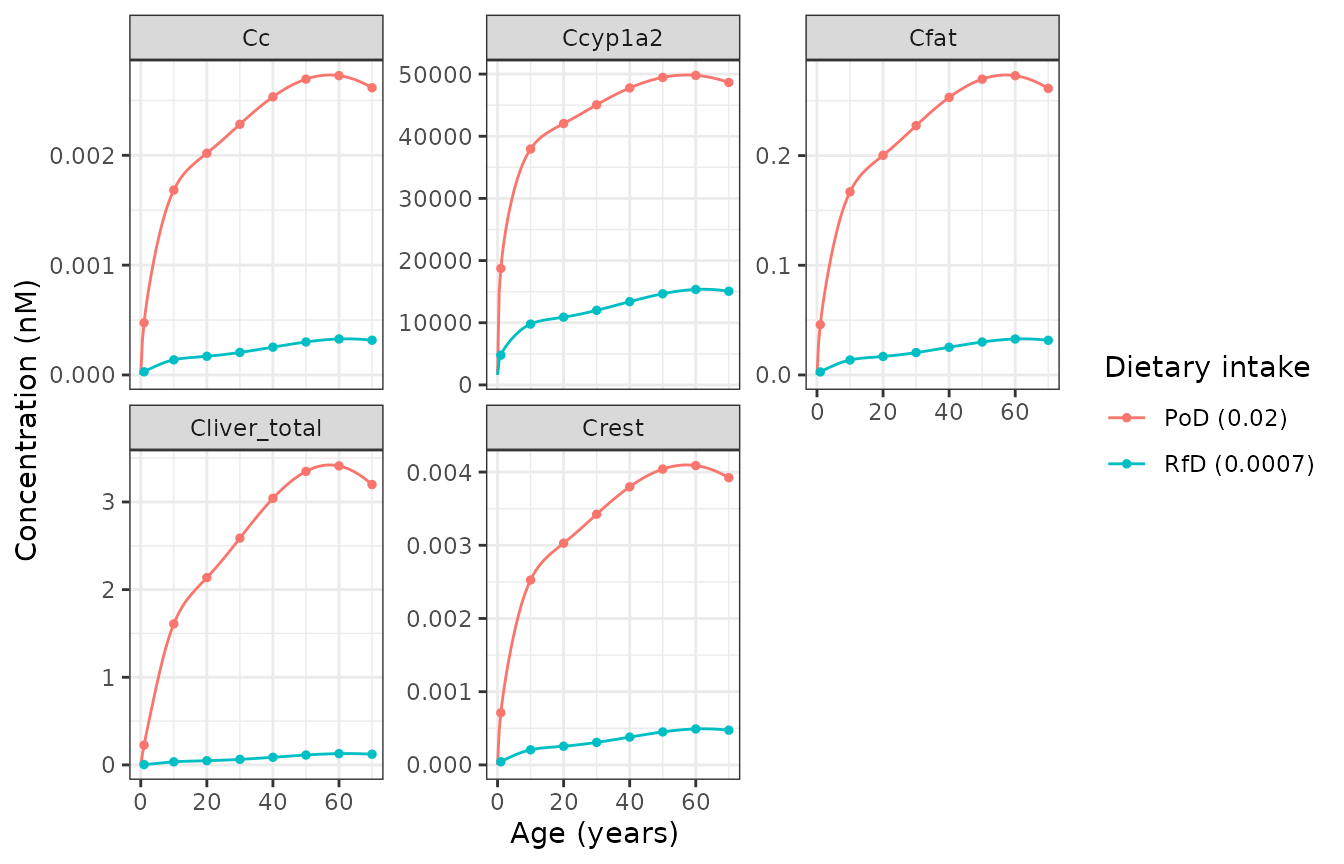
Lifetime TCDD tissue concentrations and liver CYP1A2 induction (reproduces Liu 2022 Figure 2A). Points are the authors’ Octave reference output.
Mixture cross-induction lowers extrahepatic burden (Figure 3A)
The paper’s central result: when two congeners are co-administered, shared CYP1A2 is more strongly induced than under either single exposure, which increases hepatic sequestration and metabolism and so lowers each congener’s extrahepatic (blood, fat, rest-of-body) burden relative to single exposure. The liver burden is the exception - it can rise. Below, TCDD is simulated alone and in the binary mixture with 2,3,4,7,8-PeCDF.
s_tcdd_single <- s_high # TCDD alone at PoD

# lifetime-averaged mixture:single ratio (excluding t = 0), as in the paper.
ratio <- function(mix_col, single_col) {
  m <- sb[[mix_col]][-1]
  s <- s_tcdd_single[[single_col]][-1]
  mean(m / s)
}
ratios_tcdd <- c(
  CA = ratio("Cc_tcdd", "Cc"),
  CF = ratio("Cfat_tcdd", "Cfat"),
  CRB = ratio("Crest_tcdd", "Crest"),
  CL = ratio("Cliver_total_tcdd", "Cliver_total")
)
print(round(ratios_tcdd, 3))
#>    CA    CF   CRB    CL
#> 0.817 0.817 0.817 1.020
# The paper (Section 3.2, Figure 3): CA, CF and CRB ratios are below unity
# (extrahepatic reduction); CYP1A2 is more induced in the mixture than alone.
stopifnot(
  "extrahepatic TCDD burden is reduced in the mixture" =
    all(ratios_tcdd[c("CA", "CF", "CRB")] < 1),
  "mixture induces CYP1A2 above single exposure" =
    tail(sb$Ccyp1a2, 1) > tail(s_tcdd_single$Ccyp1a2, 1)
)
cat(sprintf(
  "lifetime-end CYP1A2: single %.0f nM, binary %.0f nM\n",
  tail(s_tcdd_single$Ccyp1a2, 1), tail(sb$Ccyp1a2, 1)
))
#> lifetime-end CYP1A2: single 48650 nM, binary 62427 nM
cmp <- bind_rows(
  data.frame(year = s_tcdd_single$year, CA = s_tcdd_single$Cc,
    CL = s_tcdd_single$Cliver_total, exposure = "TCDD single"),
  data.frame(year = sb$year, CA = sb$Cc_tcdd,
    CL = sb$Cliver_total_tcdd, exposure = "TCDD in mixture")
) |>
  pivot_longer(c(CA, CL), names_to = "tissue", values_to = "conc")

ggplot(cmp, aes(year, conc, colour = exposure)) +
  geom_line() +
  facet_wrap(~tissue, scales = "free_y") +
  labs(x = "Age (years)", y = "TCDD concentration (nM)", colour = NULL) +
  theme_bw()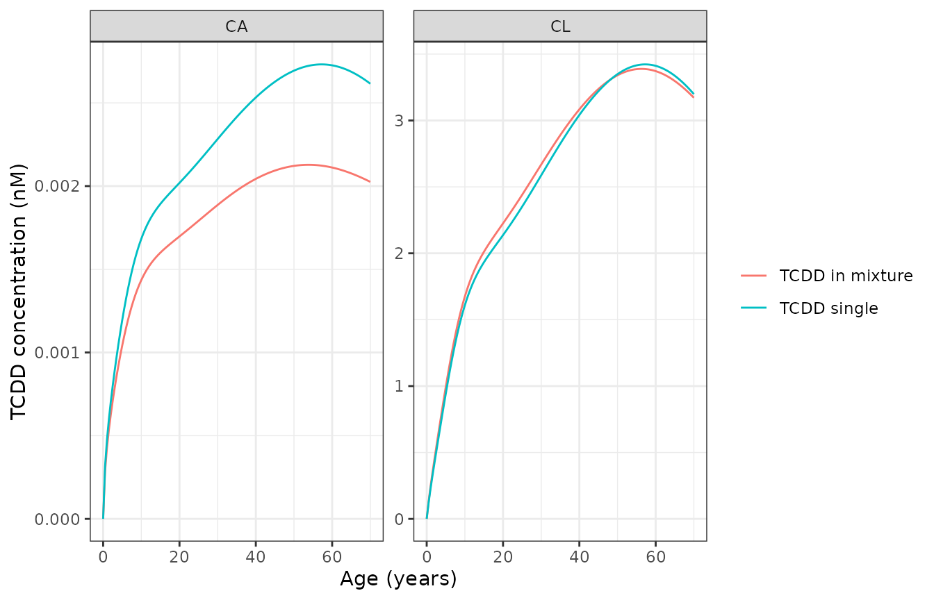
TCDD blood (CA) and total liver (CL) concentrations, single vs binary mixture with 2,3,4,7,8-PeCDF (reproduces the pattern of Liu 2022 Figure 3A): blood burden falls in the mixture while liver burden is comparable.
Full 11-congener parameter set
The framework scales to any number of congeners. The complete
chemical-specific parameter table
(DLC_human_parameters.xlsx, paper Table S3) is reproduced
below so the shipped models can be re-parameterised for any of the 11
congeners the paper studied. Columns are the liver / fat / rest-of-body
partition coefficients, the AHR dissociation constant, the hepatic
elimination rate constant, the GI absorption rate constant, molecular
weight, intake toxic equivalency factor (TEF) and systemic TEF.
congeners <- data.frame(
  congener = c("2,3,4,7,8-PeCDF", "1,2,3,7,8-PeCDF", "2,3,7,8-TCDF", "1,2,3,4,7,8-HxCDF",
    "2,3,7,8-TCDD", "1,2,3,6,7,8-HxCDF", "1,2,3,4,6,7,8-HpCDD", "1,2,3,4,6,7,8-HpCDF",
    "1,2,3,7,8-PeCDD", "1,2,3,4,6,7,8,9-OCDD", "1,2,3,4,6,7,8,9-OCDF"),
  PL = c(27.551, 11.020, 11.020, 15.306, 6.000, 27.551, 20.816, 15.918, 10.408, 34.286, 9.184),
  PF = c(136.03, 52.63, 22.27, 30.36, 100.00, 52.63, 57.89, 56.28, 174.90, 22.27, 58.30),
  PRB = c(3.167, 0.833, 0.392, 0.917, 1.500, 2.083, 3.250, 0.608, 1.583, 2.167, 0.458),
  KDAHR = c(0.149, 0.769, 0.417, 2.326, 0.100, 2.703, 2.778, 0.588, 0.333, 285.714, 62.500),
  kelim = c(6.89e-4, 7.58e-3, 1.705e-2, 1.196e-3, 1.10e-3, 1.10e-3, 1.049e-3, 2.623e-3, 7.93e-4, 1.218e-3, 3.41e-2),
  KABS = c(0.0606, 0.0612, 0.0600, 0.0600, 0.0600, 0.0600, 0.0532, 0.0538, 0.0612, 0.0470, 0.0588),
  MW = c(340.4, 340.4, 306.0, 374.9, 322.0, 374.9, 425.3, 409.3, 356.4, 459.8, 443.8),
  TEF = c(0.3, 0.03, 0.1, 0.1, 1, 0.1, 0.01, 0.01, 1, 3e-4, 3e-4),
  Systemic_TEF = c(1, 0.1, 0.1, 1, 1, 0.1, 0.1, 0.01, 1, 3e-4, 1e-3)
)
knitr::kable(congeners, digits = 4)| congener | PL | PF | PRB | KDAHR | kelim | KABS | MW | TEF | Systemic_TEF |
|---|---|---|---|---|---|---|---|---|---|
| 2,3,4,7,8-PeCDF | 27.551 | 136.03 | 3.167 | 0.149 | 0.0007 | 0.0606 | 340.4 | 3e-01 | 1e+00 |
| 1,2,3,7,8-PeCDF | 11.020 | 52.63 | 0.833 | 0.769 | 0.0076 | 0.0612 | 340.4 | 3e-02 | 1e-01 |
| 2,3,7,8-TCDF | 11.020 | 22.27 | 0.392 | 0.417 | 0.0170 | 0.0600 | 306.0 | 1e-01 | 1e-01 |
| 1,2,3,4,7,8-HxCDF | 15.306 | 30.36 | 0.917 | 2.326 | 0.0012 | 0.0600 | 374.9 | 1e-01 | 1e+00 |
| 2,3,7,8-TCDD | 6.000 | 100.00 | 1.500 | 0.100 | 0.0011 | 0.0600 | 322.0 | 1e+00 | 1e+00 |
| 1,2,3,6,7,8-HxCDF | 27.551 | 52.63 | 2.083 | 2.703 | 0.0011 | 0.0600 | 374.9 | 1e-01 | 1e-01 |
| 1,2,3,4,6,7,8-HpCDD | 20.816 | 57.89 | 3.250 | 2.778 | 0.0010 | 0.0532 | 425.3 | 1e-02 | 1e-01 |
| 1,2,3,4,6,7,8-HpCDF | 15.918 | 56.28 | 0.608 | 0.588 | 0.0026 | 0.0538 | 409.3 | 1e-02 | 1e-02 |
| 1,2,3,7,8-PeCDD | 10.408 | 174.90 | 1.583 | 0.333 | 0.0008 | 0.0612 | 356.4 | 1e+00 | 1e+00 |
| 1,2,3,4,6,7,8,9-OCDD | 34.286 | 22.27 | 2.167 | 285.714 | 0.0012 | 0.0470 | 459.8 | 3e-04 | 3e-04 |
| 1,2,3,4,6,7,8,9-OCDF | 9.184 | 58.30 | 0.458 | 62.500 | 0.0341 | 0.0588 | 443.8 | 3e-04 | 1e-03 |
Assumptions and deviations
- Parameter source. The paper’s numeric parameters live in supplements (Tables S1-S4) and in the authors’ published Octave repository. The models here are transcribed from that repository (https://github.com/pulsatility/2022-DLC-Mixture-PBPK), which the paper designates as the model source, and were validated by reproducing the Octave output to integrator tolerance (section above).
- Deterministic. The model has no IIV and no residual error; the authors’ population variability (Figure 5) comes from Monte Carlo sampling of AHR, CYP1A2 and body-weight parameters, not from estimated random effects. No error model is encoded.
-
Sex. The results the paper presents are for women,
and the shipped growth / fat-fraction polynomials are the female curves
(
g.male = 0in the Octave code). The deposit also contains male curves; they are not encoded here. - CYP1A2 intermediates. The authors replaced the Emond model’s two CYP1A2 intermediate species with an explicit mRNA step, doubling the protein half-life to preserve the induction delay (paper Section 2.3). That mRNA formulation is what is encoded.
- Fixed congener count. rxode2 has no variable-length ODE vectors, so the single-congener and binary models fix the congener count at one and two. The full 11-congener parameter set is tabulated above for re-parameterisation.
- Exposure encoding. Daily dietary intake (ng/kg bw/day) enters as a continuous zero-order input into the GI compartment computed from the time-varying body weight; there are no dose records.