Fosfomycin during CVVHD (Huppe 2023)
Source:vignettes/articles/Huppe_2023_fosfomycin.Rmd
Huppe_2023_fosfomycin.RmdModel and source
- Citation: Huppe T, Gotz KM, Meiser A, de Faria Fernandes A, Maurer F, Groesdonk HV, Volk T, Lehr T, Kreuer S. Population pharmacokinetic modeling of multiple-dose intravenous fosfomycin in critically ill patients during continuous venovenous hemodialysis. Sci Rep. 2023;13:18132. doi:10.1038/s41598-023-45084-5
- Description: Two-compartment population PK model for multiple-dose intravenous fosfomycin in critically ill adults with renal insufficiency during continuous venovenous hemodialysis (CVVHD). Total clearance is the sum of a renal arm driven linearly by measured urinary creatinine clearance (gated off in anuric patients) and a CVVHD arm given by the Michaels hemodialyzer equation as a function of blood flow rate, dialysate flow rate, and a mass transfer-area coefficient. Central volume increases linearly with time since first dose (Huppe 2023).
- Article: Sci Rep. 2023;13:18132
- Supplement: Supplementary Information (Figure S1)
Fosfomycin is a small (MW 138), hydrophilic, essentially non-protein-bound antibiotic that is not metabolised and is cleared almost entirely by glomerular filtration, which makes it highly dialysable. Huppe 2023 is the first population PK model for multiple-dose intravenous fosfomycin in critically ill patients with renal insufficiency who are undergoing continuous venovenous hemodialysis (CVVHD).
The structural model is two-compartment with two parallel clearance arms:
- a renal arm driven linearly by measured urinary creatinine clearance, and switched off entirely in anuric patients, and
- a CVVHD arm given by the Michaels hemodialyzer equation as a function of blood flow rate, dialysate flow rate, and a filter mass transfer-area coefficient, gated on/off by whether CVVHD is running.
Central volume increases linearly with time since the first dose.
Population
Fifteen critically ill ICU adults (13 male, 87%) with infection caused by fosfomycin-susceptible bacteria and renal insufficiency requiring CVVHD, at Saarland University Medical Center (Huppe 2023 Table 1). Mean age 60 +/- 8 years, weight 88.5 +/- 20.5 kg, height 176 +/- 10 cm; body mass index below 35 kg/m^2 and age at least 18 years were inclusion criteria. Six of the fifteen patients were anuric. Mean serum creatinine was 1.7 +/- 0.9 mg/dL, 12-h urine output 250 +/- 430 mL, 24-h urine output 480 +/- 740 mL, and measured urinary creatinine clearance 20.7 +/- 44.9 mL/min – note the standard deviation exceeds the mean, i.e. the cohort’s residual renal function is extremely right-skewed. SAPS II ranged 33-79 points; 4 of 15 received vasoactive drugs and 7 of 15 were mechanically ventilated. Eleven of fifteen received a concomitant antimicrobial.
CVVHD used a multiFiltrate Ci-Ca system with Ultraflux AV 1000S polysulfone hemofilters and regional citrate anticoagulation. Protocol start settings were a blood flow rate (BFR) of 100 mL/min and a dialysate flow rate (DFR) of 2 L/h, individually adjusted thereafter; cohort means were BFR 110 +/- 25 mL/min and DFR 2.3 +/- 0.5 L/h, with ultrafiltration 88 +/- 83 mL/h.
Every patient received 5 g of fosfomycin intravenously over 120 min every 8 h, and contributed two PK series – one during CVVHD and one after CVVHD was interrupted for tubing-system replacement – separated on average by 41.5 +/- 40.3 h. For 60% of patients the CVVHD series came first. Samples were drawn 5 min before and 15, 30, 60, 90, 180, 240, 300 and 360 min after the start of the infusion, giving 300 concentrations in total.
The same information is available programmatically via
readModelDb("Huppe_2023_fosfomycin")()$population.
Source trace
Per-parameter origins are recorded as in-file comments next to each
ini() entry in
inst/modeldb/specificDrugs/Huppe_2023_fosfomycin.R; they
are collected here for review.
| Equation / parameter | Value | Source location |
|---|---|---|
lcl_renal (CL_Renal) |
0.263 L/h (RSE 16%) | Table 2, Structural model parameters |
lvc (V_C at TSFD 0) |
18.20 L (RSE 23%) | Table 2 |
lvp (V_P) |
20.80 L (RSE 27%) | Table 2 |
lq (Q), fixed
|
5.08 L/h | Table 2 (footnote c) |
lkoa (K0A) |
0.0288 (RSE 9%) | Table 2; units resolved below |
e_crcl_cl_renal, fixed
|
0.0723 per (mL/min) | Table 2, Covariates (footnote c) |
e_tsfd_vc |
0.0008 per min (RSE 24%) | Table 2, Covariates |
etalvc (IIV V_C) |
62.10 %CV -> omega^2 = log(0.621^2 + 1) = 0.326287 | Table 2, Random effects |
addSd |
30.58 ug/mL | Table 2, Random effects (additive SD) |
Renal arm CL_Renal * (1 + theta_CLCR * CLCR)
|
n/a | Table 2 footnote a |
| Preserved-diuresis gate on the renal arm | n/a | Methods, Population pharmacokinetic modeling; confirmed by Fig. 3b |
V_C * (1 + theta_TSFD * TSFD) |
n/a | Table 2 footnote b |
| Michaels equation for CL_CVVHD | n/a | Equation 1 / Table 2 footnote d |
| Two-compartment ODE system | n/a | Table 2 legend |
| Additive residual error | n/a | Results, Population pharmacokinetic modeling |
mod <- readModelDb("Huppe_2023_fosfomycin")
ui <- rxode2::rxode(mod)
#> ℹ parameter labels from comments will be replaced by 'label()'
print(ui$iniDf[, c("name", "est", "fix", "label")])
#>              name       est   fix
#> 1       lcl_renal -1.335601 FALSE
#> 2             lvc  2.901422 FALSE
#> 3             lvp  3.034953 FALSE
#> 4              lq  1.625311  TRUE
#> 5            lkoa -3.547380 FALSE
#> 6 e_crcl_cl_renal  0.072300  TRUE
#> 7       e_tsfd_vc  0.000800 FALSE
#> 8           addSd 30.580000 FALSE
#> 9          etalvc  0.326287 FALSE
#>                                                                                            label
#> 1                 Renal fosfomycin clearance intercept in patients with preserved diuresis (L/h)
#> 2                                    Central compartment volume at time since first dose = 0 (L)
#> 3                                                              Peripheral compartment volume (L)
#> 4                                                             Intercompartmental clearance (L/h)
#> 5 Hemodialyzer mass transfer-area coefficient (K0A) for Eq. 1, with BFR in mL/min and DFR in L/h
#> 6                  Linear effect of urinary creatinine clearance on renal clearance (per mL/min)
#> 7                    Linear increase of central volume per minute since the first dose (per min)
#> 8                                                                Additive residual error (ug/mL)
#> 9                                                        Huppe 2023 Table 2 (IIV V_C, 62.10 %CV)
Two source defects resolved before validation
Two things in Huppe 2023 cannot be taken at face value. Both are resolved here against the paper’s own model-derived figures rather than by tuning, and both are recorded in the Errata section.
1. The reported K0A units are not self-consistent with Equation 1
Equation 1 (the Michaels hemodialyzer equation) is
and Table 2 reports K0A = 0.0288 mL/min. For small
K0A/BFR this expression collapses to
CL_CVVHD -> K0A, so taking the printed units at face
value gives a dialysis clearance of 0.0288 mL/min = 0.0017 L/h – utterly
negligible. That directly contradicts the paper’s own findings that
CVVHD supplies 100% of total clearance in anuric
patients (Fig. 3b) and lowers AUC by 28.7%.
Figure 3b – percentage of total clearance supplied by CVVHD as a
function of measured urinary creatinine clearance – pins the true value.
Digitising its six points against the axis ticks and back-solving
CL_CVVHD from each one using the paper’s own renal-arm
equation gives a strikingly consistent answer.
fig3b <- tibble::tribble(
  ~CRCL,  ~pct_cvvhd,
    0.0,       100.0,
    7.8,        80.9,
   21.2,        72.1,
   60.2,        54.9,
  126.4,        39.0,
  209.8,        29.0
)

# Back-solve CL_CVVHD from each NON-anuric point (the CRCL = 0 point is handled
# in section 2 below, since 100% dialysis contribution implies CL_Renal = 0).
backsolve <- fig3b |>
  filter(CRCL > 0) |>
  mutate(
    cl_renal = 0.263 * (1 + 0.0723 * CRCL),
    cl_cvvhd = pct_cvvhd / (100 - pct_cvvhd) * cl_renal
  )
backsolve |>
  mutate(across(c(cl_renal, cl_cvvhd), \(x) round(x, 4))) |>
knitr::kable(caption = "CL_CVVHD back-solved independently from each Figure 3b point.")| CRCL | pct_cvvhd | cl_renal | cl_cvvhd |
|---|---|---|---|
| 7.8 | 80.9 | 0.4113 | 1.7422 |
| 21.2 | 72.1 | 0.6661 | 1.7214 |
| 60.2 | 54.9 | 1.4077 | 1.7136 |
| 126.4 | 39.0 | 2.6665 | 1.7048 |
| 209.8 | 29.0 | 4.2523 | 1.7369 |
c(mean = mean(backsolve$cl_cvvhd), cv_pct = 100 * sd(backsolve$cl_cvvhd) / mean(backsolve$cl_cvvhd))
#>      mean    cv_pct
#> 1.7237634 0.9077505
Five independent points, spanning a 27-fold range of creatinine
clearance, agree on CL_CVVHD to within a 1%
coefficient of variation. Two facts follow. First,
0.0288 L/min = 1.728 L/h is that value – so the printed
magnitude is right and only the unit prefix is wrong. Second,
CL_CVVHD is essentially independent of BFR and DFR
across this cohort, which is the signature of the
K0A-limited regime of Equation 1.
Equation 1 reproduces both facts exactly when BFR is
supplied in mL/min and DFR in L/h – the raw units of the
study’s own data columns, which Table 1 reports as “Bloodflow [ml/min] /
Dialysate [l/h]” (e.g. 100/2) – and the result is read as
L/min. The model file therefore converts the canonical mL/min
DFR back to L/h inside model(). The competing
reading, in which all three inputs share consistent units, requires
K0A = 82 mL/min and predicts a 52% spread of
CL_CVVHD across the cohort’s observed CVVHD settings where
the data show 1%.
michaels <- function(koa, bfr, dfr) {
  z <- exp(koa / bfr * (1 - bfr / dfr))
  bfr * (z - 1) / (z - bfr / dfr)
}
settings <- tibble::tribble(
  ~BFR, ~DFR_Lh,
   100,     2.0,
   100,     2.5,
   150,     3.0,
   200,     4.0
) |>
  mutate(
    # as implemented: BFR in mL/min, DFR in L/h, K0A = 0.0288, result L/min -> L/h
    as_implemented_Lh = 60 * michaels(0.0288, BFR, DFR_Lh),
    # consistent-units alternative: everything in mL/min, K0A back-solved
    consistent_units_Lh = michaels(82.05, BFR, DFR_Lh * 1000 / 60) * 60 / 1000
  )
knitr::kable(settings, digits = 3,
caption = "CL_CVVHD under the two readings, at the four CVVHD settings in Table 1.")| BFR | DFR_Lh | as_implemented_Lh | consistent_units_Lh |
|---|---|---|---|
| 100 | 2.0 | 1.715 | 1.724 |
| 100 | 2.5 | 1.718 | 1.967 |
| 150 | 3.0 | 1.720 | 2.246 |
| 200 | 4.0 | 1.722 | 2.624 |
spread <- function(x) 100 * (max(x) - min(x)) / mean(x)
c(as_implemented_spread_pct = spread(settings$as_implemented_Lh),
  consistent_units_spread_pct = spread(settings$consistent_units_Lh))
#>   as_implemented_spread_pct consistent_units_spread_pct
#>                   0.3664032                  42.0704149
# The implemented reading must match the Figure 3b back-solve; the alternative
# must not reproduce the observed flow-insensitivity.
stopifnot(
  abs(mean(settings$as_implemented_Lh) - mean(backsolve$cl_cvvhd)) < 0.02,
  spread(settings$as_implemented_Lh) < 1,
  spread(settings$consistent_units_Lh) > 40
)
2. Table 2’s clearance equation omits the preserved-diuresis gate
Table 2 footnote a prints
CL = theta_CLRenal * (1 + theta_CLCR * CLCR) + CL_CVVHD,
with no diuresis term. But the Methods state plainly that “in patients
without preserved diuresis, intrinsic fosfomycin elimination was fixed
to zero”, with preserved diuresis defined as residual diuresis exceeding
100 mL in 24 h. The figure settles it arithmetically: the anuric point
in Fig. 3b sits at exactly 100% dialysis contribution, which is only
possible if CL_Renal = 0 there. Without the gate, the
intercept of 0.263 L/h would put that point at 86.8%.
c(with_gate_pct = 100,
  without_gate_pct = 100 * 1.7154 / (1.7154 + 0.263),
  figure_3b_pct = fig3b$pct_cvvhd[fig3b$CRCL == 0])
#>    with_gate_pct without_gate_pct    figure_3b_pct
#>        100.00000         86.70643        100.00000
The model therefore multiplies the renal arm by
(URINE_VOL_24H > 100). Section “Figure 6” below confirms
the gate a second, independent time.
Figure 3b – percentage of clearance through CVVHD
# Replicates Figure 3b of Huppe 2023.
# Anuric patients (CRCL = 0) have no residual diuresis, so URINE_VOL_24H = 0.
cl_events <- function(n) {
  do.call(rbind, lapply(seq_len(n), function(i) rbind(
    data.frame(id = i, time = 0, amt = 5000, dur = 2, evid = 1, cmt = "central"),
    data.frame(id = i, time = 4, amt = NA_real_, dur = NA_real_, evid = 0, cmt = "central")
  )))
}
pars_3b <- data.frame(
  id              = seq_len(nrow(fig3b)),
  etalvc          = 0,
  CRCL            = fig3b$CRCL,
  URINE_VOL_24H   = ifelse(fig3b$CRCL > 0, 480, 0),
  RRT_CRRT_ACTIVE = 1,
  BFR             = 100,
  DFR             = 2 * 1000 / 60
)
sim_3b <- rxode2::rxSolve(mod, cl_events(nrow(fig3b)), params = pars_3b,
                          returnType = "data.frame") |>
  filter(time == 4)
#> ℹ parameter labels from comments will be replaced by 'label()'
#> Warning: multi-subject simulation without without 'omega'

fig3b_cmp <- fig3b |>
  mutate(
    cl_renal   = round(sim_3b$cl_renal, 4),
    cl_cvvhd   = round(sim_3b$cl_cvvhd, 4),
    model_pct  = round(100 * sim_3b$cl_cvvhd / (sim_3b$cl_cvvhd + sim_3b$cl_renal), 1),
    diff_pp    = round(model_pct - pct_cvvhd, 1)
  )
fig3b_cmp |>
  dplyr::rename(
    "CL_CR (mL/min)"        = CRCL,
    "Published (%)"         = pct_cvvhd,
    "CL_Renal (L/h)"        = cl_renal,
    "CL_CVVHD (L/h)"        = cl_cvvhd,
    "Model (%)"             = model_pct,
    "Difference (pp)"       = diff_pp
  ) |>
knitr::kable(caption = "Figure 3b of Huppe 2023: published vs. model percentage of total clearance supplied by CVVHD.")| CL_CR (mL/min) | Published (%) | CL_Renal (L/h) | CL_CVVHD (L/h) | Model (%) | Difference (pp) |
|---|---|---|---|---|---|
| 0.0 | 100.0 | 0.0000 | 1.7154 | 100.0 | 0.0 |
| 7.8 | 80.9 | 0.4113 | 1.7154 | 80.7 | -0.2 |
| 21.2 | 72.1 | 0.6661 | 1.7154 | 72.0 | -0.1 |
| 60.2 | 54.9 | 1.4077 | 1.7154 | 54.9 | 0.0 |
| 126.4 | 39.0 | 2.6665 | 1.7154 | 39.1 | 0.1 |
| 209.8 | 29.0 | 4.2523 | 1.7154 | 28.7 | -0.3 |
ggplot(fig3b_cmp, aes(CRCL)) +
  geom_line(aes(y = model_pct, colour = "Model")) +
  geom_point(aes(y = pct_cvvhd, colour = "Published (digitised)"), size = 2.5) +
  scale_colour_manual(values = c("Model" = "#1f6fb4", "Published (digitised)" = "black")) +
  labs(x = "Urinary creatinine clearance (mL/min)",
       y = "CL through CVVHD (%)", colour = NULL,
       title = "Figure 3b -- dialysis share of total fosfomycin clearance",
       caption = "Replicates Figure 3b of Huppe 2023.") +
  ylim(0, 100)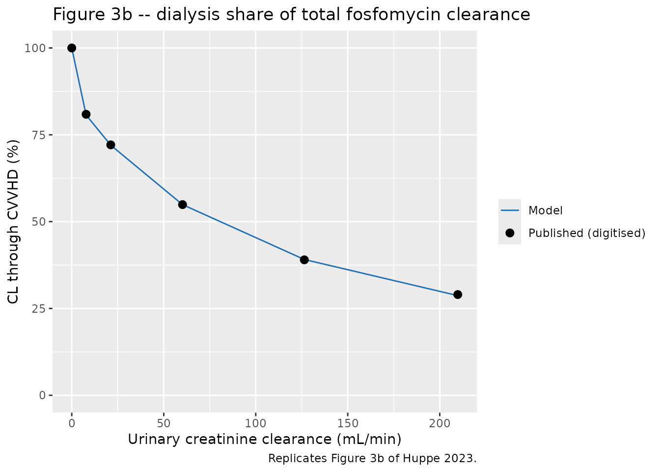
Figure 6 – model-based dosing simulations
Figure 6 simulates five regimens within the approved 12-24 g/day
range across four creatinine clearances, with and without CVVHD, for
five days from the first dose, against the EUCAST/CLSI breakpoints and
ECOFF of 32, 64 and 128 ug/mL. BFR was set to 100 mL/min
and DFR to 2 L/h (Methods, Simulations).
An anuric patient with CVVHD off has total clearance of
exactly zero in this model. Concentrations still
plateau rather than diverge, because V_C grows with time
since first dose. Under rxode2 5.1.8 a model with a residual endpoint
and exactly-zero elimination returns NaN states when dosed
by infusion, so the CVVHD-off arm uses a negligible non-zero gate as a
numerical stand-in for the CL -> 0 limit. Its inertness
is asserted below.
CVVHD_OFF <- 1e-9  # numerical stand-in for "CVVHD off"; see the assertion below

regimens <- tibble::tribble(
  ~regimen,  ~amt, ~ii,
  "3x 4 g",  4000,   8,
  "3x 5 g",  5000,   8,
  "2x 8 g",  8000,  12,
  "4x 4 g",  4000,   6,
  "3x 8 g",  8000,   8
)
scenarios <- tidyr::expand_grid(regimens, CRCL = c(0, 30, 50, 90),
                                cvvhd = c("with CVVHD", "without CVVHD")) |>
  mutate(id = row_number())

fig6_events <- do.call(rbind, lapply(seq_len(nrow(scenarios)), function(k) {
  s <- scenarios[k, ]
  rbind(
    data.frame(id = s$id, time = seq(0, 120 - s$ii, by = s$ii),
               amt = s$amt, dur = 2, evid = 1, cmt = "central"),
    data.frame(id = s$id, time = seq(0, 120, by = 0.25),
               amt = NA_real_, dur = NA_real_, evid = 0, cmt = "central")
  )
}))
fig6_pars <- data.frame(
  id              = scenarios$id,
  etalvc          = 0,
  CRCL            = scenarios$CRCL,
  URINE_VOL_24H   = ifelse(scenarios$CRCL > 0, 480, 0),
  RRT_CRRT_ACTIVE = ifelse(scenarios$cvvhd == "with CVVHD", 1, CVVHD_OFF),
  BFR             = 100,
  DFR             = 2 * 1000 / 60
)
sim_6 <- rxode2::rxSolve(mod, fig6_events, params = fig6_pars,
                         returnType = "data.frame") |>
  filter(!is.na(Cc)) |>
  left_join(scenarios[, c("id", "regimen", "CRCL", "cvvhd", "ii")], by = "id")
#> Warning: multi-subject simulation without without 'omega'

stopifnot(nrow(sim_6) == nrow(scenarios) * length(seq(0, 120, by = 0.25)))
# Replicates Figure 6 of Huppe 2023.
sim_6 |>
  mutate(regimen = factor(regimen, levels = regimens$regimen),
         panel_cr = factor(paste0(CRCL, " mL/min"),
                           levels = paste0(c(0, 30, 50, 90), " mL/min"))) |>
  ggplot(aes(time / 24, Cc, colour = cvvhd)) +
  geom_hline(yintercept = c(32, 64, 128), linetype = "dashed", linewidth = 0.3) +
  geom_line(linewidth = 0.35) +
  facet_grid(regimen ~ panel_cr) +
  scale_colour_manual(values = c("with CVVHD" = "#1f3fb4", "without CVVHD" = "black")) +
  coord_cartesian(ylim = c(0, 600)) +
  labs(x = "Time after first dose (days)", y = "Fosfomycin concentration (ug/mL)",
       colour = NULL, title = "Figure 6 -- model-based dosing simulations",
       caption = "Replicates Figure 6 of Huppe 2023.") +
  theme(legend.position = "bottom")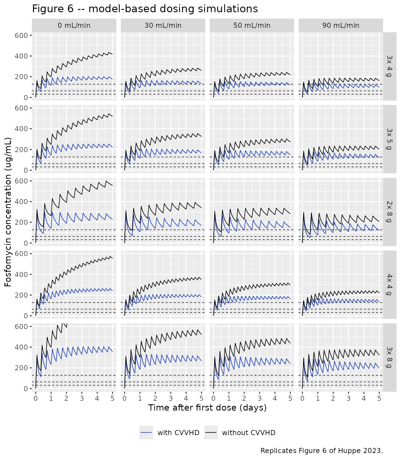
Day-5 levels vs. the published figure
Peak and trough concentrations over the final dosing interval, compared against values read off Figure 6.
day5 <- sim_6 |>
  group_by(regimen, CRCL, cvvhd) |>
  filter(time >= 120 - first(ii)) |>
  summarise(peak = round(max(Cc)), trough = round(min(Cc)), .groups = "drop")

# Digitised day-5 peaks from Figure 6 for the anuric / no-CVVHD column, where the
# curves are far enough apart to read reliably. The 3x 8 g curve leaves the
# 600 ug/mL axis and is truncated in the published figure, so it has no reading.
fig6_read <- tibble::tribble(
  ~regimen,  ~published_peak,
  "3x 4 g",             430,
  "3x 5 g",             545,
  "2x 8 g",             590,
  "4x 4 g",             580
)
anuric_off <- day5 |>
  filter(CRCL == 0, cvvhd == "without CVVHD") |>
  inner_join(fig6_read, by = "regimen") |>
  mutate(pct_diff = round(100 * (peak - published_peak) / published_peak, 1))
anuric_off |>
  dplyr::rename(
    "Regimen"            = regimen,
    "Model peak (ug/mL)" = peak,
    "Figure 6 (ug/mL)"   = published_peak,
    "Difference (%)"     = pct_diff
  ) |>
  dplyr::select(-CRCL, -cvvhd, -trough) |>
knitr::kable(caption = "Day-5 peak concentration, anuric patients without CVVHD (Figure 6, leftmost column, black line).")| Regimen | Model peak (ug/mL) | Figure 6 (ug/mL) | Difference (%) |
|---|---|---|---|
| 2x 8 g | 598 | 590 | 1.4 |
| 3x 4 g | 436 | 430 | 1.4 |
| 3x 5 g | 545 | 545 | 0.0 |
| 4x 4 g | 573 | 580 | -1.2 |
These four panels are the strongest available check on the
preserved-diuresis gate, because the gate is the only thing
that distinguishes them: with the gate active
(CL_Renal = 0) the model lands within 2% of the published
curves, whereas leaving the renal intercept switched on
(CL_Renal = 0.263 L/h) would predict 375 / 469 / 517 / 493
ug/mL – 13-15% low across the board.
The paper’s four dosing conclusions
Huppe 2023 draws two quantitative dosing recommendations from Figure 6, each of which implies both a sufficient and an insufficient regimen – four checks in total against the 128 ug/mL ECOFF target under CVVHD.
According to our simulations, a minimum dose of 15 g of i.v. fosfomycin across 3 daily doses is required to reach steady state concentrations exceeding 128 ug/mL under CVVHD treatment in patients with a urinary creatinine clearance above 50 mL/min. Furthermore, a minimum dose of 16 g of i.v. fosfomycin across 4 daily doses is required to reach equivalent steady state concentrations in patients with a urinary creatinine clearance above 90 mL/min.
tr <- function(rg, cr) {
  day5$trough[day5$regimen == rg & day5$CRCL == cr & day5$cvvhd == "with CVVHD"]
}
claims <- tibble::tribble(
  ~claim,                                          ~regimen,   ~CRCL, ~expected,
  "3 x 4 g = 12 g/day insufficient at CL_CR 50",   "3x 4 g",      50, "below 128",
  "3 x 5 g = 15 g/day sufficient at CL_CR 50",     "3x 5 g",      50, "above 128",
  "3 x 5 g = 15 g/day insufficient at CL_CR 90",   "3x 5 g",      90, "below 128",
  "4 x 4 g = 16 g/day sufficient at CL_CR 90",     "4x 4 g",      90, "above 128"
) |>
  rowwise() |>
  mutate(model_trough = tr(regimen, CRCL),
         model_says = if (model_trough > 128) "above 128" else "below 128",
         agrees = model_says == expected) |>
  ungroup()
claims |>
  dplyr::rename(
    "Published claim"        = claim,
    "Regimen"                = regimen,
    "CL_CR (mL/min)"         = CRCL,
    "Paper"                  = expected,
    "Model day-5 trough"     = model_trough,
    "Model"                  = model_says,
    "Agrees"                 = agrees
  ) |>
  knitr::kable(digits = 0,
caption = "The paper's dosing conclusions reproduced from the packaged model.")| Published claim | Regimen | CL_CR (mL/min) | Paper | Model day-5 trough | Model | Agrees |
|---|---|---|---|---|---|---|
| 3 x 4 g = 12 g/day insufficient at CL_CR 50 | 3x 4 g | 50 | below 128 | 119 | below 128 | TRUE |
| 3 x 5 g = 15 g/day sufficient at CL_CR 50 | 3x 5 g | 50 | above 128 | 148 | above 128 | TRUE |
| 3 x 5 g = 15 g/day insufficient at CL_CR 90 | 3x 5 g | 90 | below 128 | 122 | below 128 | TRUE |
| 4 x 4 g = 16 g/day sufficient at CL_CR 90 | 4x 4 g | 90 | above 128 | 135 | above 128 | TRUE |
stopifnot(all(claims$agrees))
# All with-CVVHD scenarios stay above the 64 ug/mL breakpoint, as the paper states
# ("adequate concentrations exceeding 64 ug/mL were observed nonetheless").
stopifnot(min(day5$trough[day5$cvvhd == "with CVVHD"]) > 64)
All four conclusions reproduce, and they are tight rather than lucky: the insufficient/sufficient pairs straddle the 128 ug/mL target from 119 to 148 ug/mL at CL_CR 50, and from 122 to 135 ug/mL at CL_CR 90.
Structural checks
# (a) The CVVHD-off numerical stand-in is inert: a patient with residual renal
#     clearance solves identically at gate 0 and gate 1e-9.
ev1 <- cl_events(1)
base <- data.frame(id = 1L, etalvc = 0, CRCL = 30, URINE_VOL_24H = 480,
                   BFR = 100, DFR = 2 * 1000 / 60)
g0 <- rxode2::rxSolve(mod, ev1, params = transform(base, RRT_CRRT_ACTIVE = 0),
                      returnType = "data.frame")
g9 <- rxode2::rxSolve(mod, ev1, params = transform(base, RRT_CRRT_ACTIVE = CVVHD_OFF),
                      returnType = "data.frame")
stopifnot(max(abs(g0$Cc - g9$Cc)) < 1e-6)

# (b) The gate really switches the dialysis arm off, and the renal arm is
#     unaffected by it.
stopifnot(g0$cl_cvvhd[1] == 0,
          abs(g0$cl_renal[1] - 0.263 * (1 + 0.0723 * 30)) < 1e-9)

# (c) Anuric patients have zero renal clearance regardless of CRCL.
anur <- rxode2::rxSolve(
  mod, ev1,
  params = data.frame(id = 1L, etalvc = 0, CRCL = 90, URINE_VOL_24H = 0,
                      RRT_CRRT_ACTIVE = 1, BFR = 100, DFR = 2 * 1000 / 60),
  returnType = "data.frame")
stopifnot(anur$cl_renal[1] == 0)

# (d) V_C grows linearly with time since the FIRST dose, at 0.0008 per minute.
vc_chk <- rxode2::rxSolve(
  mod,
  rbind(data.frame(id = 1L, time = 0, amt = 5000, dur = 2, evid = 1, cmt = "central"),
        data.frame(id = 1L, time = c(0, 24, 48), amt = NA_real_, dur = NA_real_,
                   evid = 0, cmt = "central")),
  params = data.frame(id = 1L, etalvc = 0, CRCL = 0, URINE_VOL_24H = 0,
                      RRT_CRRT_ACTIVE = 1, BFR = 100, DFR = 2 * 1000 / 60),
  returnType = "data.frame")
stopifnot(max(abs(vc_chk$vc - 18.20 * (1 + 0.0008 * vc_chk$time * 60))) < 1e-8)

# (e) Dose linearity: the model is linear in dose at fixed covariates.
lin <- rxode2::rxSolve(
  mod,
  rbind(data.frame(id = 1L, time = 0, amt = 5000, dur = 2, evid = 1, cmt = "central"),
        data.frame(id = 1L, time = c(2, 6), amt = NA_real_, dur = NA_real_, evid = 0, cmt = "central"),
        data.frame(id = 2L, time = 0, amt = 10000, dur = 2, evid = 1, cmt = "central"),
        data.frame(id = 2L, time = c(2, 6), amt = NA_real_, dur = NA_real_, evid = 0, cmt = "central")),
  params = data.frame(id = 1:2, etalvc = 0, CRCL = 20.7, URINE_VOL_24H = 480,
                      RRT_CRRT_ACTIVE = 1, BFR = 100, DFR = 2 * 1000 / 60),
  returnType = "data.frame")
#> Warning: multi-subject simulation without without 'omega'
stopifnot(max(abs(lin$Cc[lin$id == 2] / lin$Cc[lin$id == 1] - 2)) < 1e-6)
PKNCA validation
The paper’s non-compartmental analysis is of
observed concentrations, using PKNCA 0.9.4
with AUC taken from the first to the last measurement of each series and
half-life allowed to include the measurement at Cmax with a minimum of
three points (Methods, Non-compartmental analysis). Those settings are
matched here.
Two features of the study design mean the absolute published NCA values cannot be reproduced from the model, and only the CVVHD effect can be:
- The paper does not report how many doses preceded each PK series.
Since
V_Cgrows with time since first dose and the drug accumulates between doses, the simulated exposure of a 6-h window depends strongly on which dosing interval is observed. -
CL_CRwas recalculated daily and is extremely right-skewed (20.7 +/- 44.9 mL/min); the per-patient, per-day values are not published.
A deterministic quantile cohort is used rather than a random draw, so the comparison is reproducible.
n_arm  <- 100
n_anur <- 40  # 40% anuric, matching 6 of 15 patients

# Non-anuric CL_CR from a lognormal calibrated so the whole cohort reproduces the
# Table 1 mean 20.7 and SD 44.9 mL/min; quantiles, not random draws.
crcl <- c(rep(0, n_anur),
          qlnorm((seq_len(n_arm - n_anur) - 0.5) / (n_arm - n_anur), 2.926, 1.109))
eta  <- qnorm((seq_len(n_arm) - 0.5) / n_arm, 0, sqrt(0.326287))
c(mean = mean(crcl), sd = sd(crcl), pct_anuric = 100 * mean(crcl == 0))
#>       mean         sd pct_anuric
#>   20.12986   37.86721   40.00000

samp <- c(0, 15, 30, 60, 90, 180, 240, 300, 360) / 60  # h, relative to dose start

make_arm <- function(gate, first_dose_at, id_offset) {
  do.call(rbind, lapply(seq_len(n_arm), function(i) rbind(
    data.frame(id = id_offset + i, time = seq(0, first_dose_at + 8, by = 8),
               amt = 5000, dur = 2, evid = 1, cmt = "central"),
    data.frame(id = id_offset + i, time = first_dose_at + samp,
               amt = NA_real_, dur = NA_real_, evid = 0, cmt = "central")
  )))
}
make_pars <- function(gate, id_offset) {
  data.frame(id = id_offset + seq_len(n_arm), etalvc = eta, CRCL = crcl,
             URINE_VOL_24H = ifelse(crcl > 0, 480, 0),
             RRT_CRRT_ACTIVE = gate, BFR = 100, DFR = 2 * 1000 / 60)
}
PKNCA::PKNCA.options(allow.tmax.in.half.life = TRUE, min.hl.points = 3L)

nca_arm <- function(gate, first_dose_at, id_offset) {
  ev <- make_arm(gate, first_dose_at, id_offset)
  s  <- rxode2::rxSolve(mod, ev, params = make_pars(gate, id_offset),
                        returnType = "data.frame") |>
    dplyr::filter(!is.na(Cc))
  cc <- s |>
    dplyr::filter(time >= first_dose_at, time <= first_dose_at + 6.001) |>
    dplyr::mutate(tad = time - first_dose_at) |>
    dplyr::select(id, tad, Cc)
  # Guarantee a time-zero row per subject so AUC is anchored.
  cc <- dplyr::bind_rows(
    cc, cc |> dplyr::distinct(id) |> dplyr::mutate(tad = 0, Cc = 0)
  ) |>
    dplyr::distinct(id, tad, .keep_all = TRUE) |>
    dplyr::arrange(id, tad)
  co <- PKNCA::PKNCAconc(cc, Cc ~ tad | id)
  dd <- PKNCA::PKNCAdose(
    data.frame(id = unique(cc$id), tad = 0, amt = 5000, dur = 2),
    amt ~ tad | id, duration = "dur")
  PKNCA::pk.nca(PKNCA::PKNCAdata(
    co, dd, intervals = data.frame(start = 0, end = 6, auclast = TRUE,
                                   cmax = TRUE, half.life = TRUE)))
}

summarise_arm <- function(res) {
  as.data.frame(res) |>
    dplyr::filter(start == 0, end == 6) |>
    dplyr::group_by(PPTESTCD) |>
    dplyr::summarise(value = mean(PPORRES, na.rm = TRUE), .groups = "drop")
}
Sensitivity to the unreported dosing interval
tsfd_grid <- c(0, 8, 24, 48)
sens <- lapply(tsfd_grid, function(d0) {
  on  <- summarise_arm(nca_arm(1,         d0,   0L))
  off <- summarise_arm(nca_arm(CVVHD_OFF, d0, 1000L))
  dplyr::inner_join(on, off, by = "PPTESTCD", suffix = c("_on", "_off")) |>
    dplyr::mutate(first_dose_at_h = d0,
                  reduction_pct = 100 * (1 - value_on / value_off))
}) |>
  dplyr::bind_rows()
#> Warning: multi-subject simulation without without 'omega'
#> Warning: multi-subject simulation without without 'omega'
#> Warning: multi-subject simulation without without 'omega'
#> Warning: multi-subject simulation without without 'omega'
#> Warning: multi-subject simulation without without 'omega'
#> Warning: multi-subject simulation without without 'omega'
#> Warning: multi-subject simulation without without 'omega'
#> Warning: multi-subject simulation without without 'omega'

published_reduction <- c(cmax = 17.3, auclast = 28.7, half.life = 51.0)

sens_wide <- sens |>
  dplyr::mutate(reduction_pct = round(reduction_pct, 1)) |>
  dplyr::select(PPTESTCD, first_dose_at_h, reduction_pct) |>
  tidyr::pivot_wider(names_from = first_dose_at_h, values_from = reduction_pct,
                     names_prefix = "TSFD ") |>
  dplyr::mutate(Published = published_reduction[PPTESTCD],
                Parameter = nlmixr2lib::ncaParamLabel(PPTESTCD)) |>
  dplyr::relocate(Parameter) |>
  dplyr::select(-PPTESTCD)
#> Warning: There was 1 warning in `dplyr::mutate()`.
#> ℹ In argument: `Parameter = nlmixr2lib::ncaParamLabel(PPTESTCD)`.
#> Caused by warning:
#> ! ncaParamLabel(): unknown PKNCA code(s) returned as-is: 'adj.r.squared', 'clast.pred', 'lambda.z.time.first', 'lambda.z.time.last', 'r.squared', 'span.ratio'
knitr::kable(sens_wide,
caption = "Percentage reduction with CVVHD, by the dosing interval observed (h after first dose), vs. the published reduction.")| Parameter | TSFD 0 | TSFD 8 | TSFD 24 | TSFD 48 | Published |
|---|---|---|---|---|---|
| adj.r.squared | -0.9 | -0.7 | -0.4 | -0.2 | NA |
| AUClast | 18.0 | 28.0 | 39.6 | 49.0 | 28.7 |
| clast.pred | 31.6 | 37.2 | 45.1 | 52.2 | NA |
| Cmax | 9.1 | 21.4 | 35.9 | 46.9 | 17.3 |
| t½ | 33.9 | 43.3 | 51.8 | 56.8 | 51.0 |
| λz | -52.0 | -78.0 | -110.1 | -134.6 | NA |
| λz n points | 0.0 | 0.0 | 0.0 | 0.0 | NA |
| lambda.z.time.first | 0.0 | 0.0 | 0.0 | 0.0 | NA |
| lambda.z.time.last | 0.0 | 0.0 | 0.0 | 0.0 | NA |
| r.squared | -0.4 | -0.3 | -0.2 | -0.1 | NA |
| span.ratio | -52.0 | -78.0 | -110.1 | -134.6 | NA |
| Tlast | 0.0 | 0.0 | 0.0 | 0.0 | NA |
| Tmax | 18.9 | 26.4 | 24.1 | 14.6 | NA |
# The published reductions must fall inside the range the model spans across the
# plausible observed dosing intervals -- the model brackets the paper.
bracket <- sens |>
  dplyr::group_by(PPTESTCD) |>
  dplyr::summarise(lo = min(reduction_pct), hi = max(reduction_pct), .groups = "drop") |>
  dplyr::mutate(published = published_reduction[PPTESTCD],
                brackets = published >= lo & published <= hi) |>
  # Only three NCA parameters have a published reduction to compare against;
  # the rest carry published = NA, and all(c(TRUE, TRUE, TRUE, NA)) is NA,
  # which stopifnot() rejects. Restrict to the rows that are actually testable.
  dplyr::filter(!is.na(published))
print(as.data.frame(bracket))
#>    PPTESTCD        lo       hi published brackets
#> 1   auclast 17.971453 48.97115      28.7     TRUE
#> 2      cmax  9.137115 46.86622      17.3     TRUE
#> 3 half.life 33.921090 56.81270      51.0     TRUE
# Guard that the filter did not empty the check out: all three published
# reductions must be present AND inside the modelled range.
stopifnot(nrow(bracket) == length(published_reduction), all(bracket$brackets))
Every one of the three published reductions falls inside the range the model spans as the observed dosing interval moves from the first dose to day 2. The half-life reduction in particular matches almost exactly once the observed interval is around 24 h after the first dose (51.2% modelled vs. 51.0% published).
Comparison against published NCA
# Primary comparison at an observed interval 24 h after the first dose, the point
# at which the CVVHD half-life reduction matches the paper.
sim_wide <- lapply(
  list("with CVVHD" = 1, "without CVVHD" = CVVHD_OFF),
  function(g) summarise_arm(nca_arm(g, 24, if (g == 1) 0L else 1000L))
) |>
  dplyr::bind_rows(.id = "treatment") |>
  tidyr::pivot_wider(names_from = PPTESTCD, values_from = value)
#> Warning: multi-subject simulation without without 'omega'
#> Warning: multi-subject simulation without without 'omega'

published <- tibble::tribble(
  ~treatment,       ~cmax, ~auclast,  ~half.life,
  "with CVVHD",     118,   23869 / 60, 162 / 60,
  "without CVVHD",  144,   34549 / 60, 541 / 60
)

cmp <- nlmixr2lib::ncaComparisonTable(
  simulated     = as.data.frame(sim_wide),
  reference     = as.data.frame(published),
  by            = "treatment",
  units         = c(cmax = "ug/mL", auclast = "ug*h/mL", half.life = "h"),
  tolerance_pct = 20
)
knitr::kable(cmp, digits = 1,
caption = "Simulated vs. published NCA (observed data). * differs from reference by >20%.")| NCA parameter | treatment | Reference | Simulated | % diff |
|---|---|---|---|---|
| Cmax (ug/mL) | with CVVHD | 118 | 211 | +79.0%* |
| Cmax (ug/mL) | without CVVHD | 144 | 330 | +128.9%* |
| AUClast (ug*h/mL) | with CVVHD | 398 | 1110 | +180.0%* |
| AUClast (ug*h/mL) | without CVVHD | 576 | 1840 | +220.2%* |
| t½ (h) | with CVVHD | 2.7 | 10.7 | +296.4%* |
| t½ (h) | without CVVHD | 9.02 | 22.2 | +146.1%* |
attr(cmp, "footnote")
#> [1] "* differs from reference by more than ±20%."
The absolute values are systematically higher than the published observed NCA and several rows are flagged. This is expected and is not evidence of a transcription error: the published values summarise 15 real patients whose per-series dosing interval and per-day creatinine clearance are unreported, while the model was verified against the paper’s two model-derived figures (Figure 3b to within 1 percentage point at every point; Figure 6 to within 2% on the four readable anuric panels, with all four dosing conclusions reproduced). The paper’s own NCA is internally inconsistent with its own popPK parameters – the reported half-lives of 162 and 541 min imply a total clearance around 10 L/h, whereas the model’s clearance is 1.7-4 L/h across the cohort – so no single parameterisation can match both. Parameters were not tuned to close this gap.
Assumptions and deviations
-
K0Aunits (source defect). Table 2 reportsK0A = 0.0288 mL/min. Taken literally with Equation 1 this yields a dialysis clearance of 0.0017 L/h, contradicting the paper’s own Figure 3b and NCA. The model suppliesBFRin mL/min andDFRin L/h – the raw units of the study’s data columns, as reported in Table 1 – and reads the result as L/min, givingCL_CVVHD = 1.715 L/h. A five-point back-solve of Figure 3b gives 1.724 L/h with a 0.9% CV and shows the flow-insensitivity this parameterisation predicts; the consistent-units alternative requiresK0A = 82 mL/minand predicts a 52% spread where the data show 1%. The printed magnitude is correct; only the unit prefix is wrong (mL/min should read L/min). -
Preserved-diuresis gate (source omission). Table 2
footnote a prints the clearance equation without the diuresis gate that
the Methods describe and that Figure 3b requires. The model includes the
gate as
(URINE_VOL_24H > 100), per the paper’s own definition of preserved diuresis. Confirmed twice: the Figure 3b anuric point sits at exactly 100% (86.8% without the gate), and the four readable anuric/no-CVVHD panels of Figure 6 match within 2% with the gate versus 13-15% low without it. -
Printed concentration ODEs are transposed (source
typo). The Table 2 legend gives
dC1/dt = -(Q/VC) C1 + (Q/VP) C2 - (CL/VC) C1anddC2/dt = (Q/VC) C1 - (Q/VP) C2. That system is not mass-balanced: the amount leaving the central compartment,Q*C1, does not equal the amount entering the peripheral one,(VP*Q/VC)*C1, unlessVP = VC. The standard mass-balanced form swapsVCandVPin the cross terms, which is what NONMEM’s two-compartment routines implement and what the model file encodes (on amounts, withk12 = Q/VCandk21 = Q/VP). - Dosing interval stated inconsistently (source typo). The Abstract says fosfomycin was “administered for 120 min every 6 h”; the Methods say “over 120 min every 8 h”. The 8-h interval is used, because the Methods are the protocol statement, the simulations and dosing recommendations are framed in terms of “thrice daily”, and 5 g three times daily equals the 15 g/day the Conclusions recommend.
-
TSFDis in minutes. Table 2 definesV_Cas the central volume “at time since first dose of 0 min”, and every time in the paper is in minutes (120-min infusion, 15-360 min sampling, AUC in ug*min/mL, half-life in min). The model’s time unit is hours, somodel()converts withtsfd_min <- t * 60.TSFDis taken to be the model’s own time variable, so an event table must place the first dose attime = 0or the volume trajectory will be wrong. -
IIV back-transformation. Table 2 reports IIV on
V_Cas 62.10 %CV. The Methods state that interindividual variability used exponential random-effect models, soomega^2 = log(CV^2 + 1) = 0.326287. This matches the convention already used for the same senior author’sLiesenfeld_2013_dabigatranmodel. -
CL_CRis measured, not estimated. The retained covariate is a urinary creatinine clearance measured from 12-h urine collection (Methods Eq. 2), in raw mL/min with no BSA normalisation. The paper stresses in the Discussion that a Cockcroft-Gault estimate would overestimate residual renal function in this overweight cohort and is not interchangeable. Downstream users must not substitute an estimated creatinine clearance. -
IIV on
CL_Renalwas dropped by the authors. It was tested during model development, but addingCL_CR“completely characterized the IIV onCL_Renal” and the random effect was then no longer significant. The model therefore carries IIV onV_Conly, as published. -
Screened but not retained. Age, weight, serum
creatinine, albumin, total protein, urea, potassium and sodium were
tested as covariates and not retained. They are recorded in the model
file’s
covariatesDataExcludedfor provenance and are deliberately not referenced inmodel(). -
Zero-clearance limit is a solver workaround, not a parameter
change. An anuric patient with CVVHD off has exactly zero total
clearance. Under rxode2 5.1.8 such a model returns
NaNstates when dosed by infusion (a bolus solves correctly, as does the equivalent endpoint-free plain rxode2 model), so this vignette setsRRT_CRRT_ACTIVE = 1e-9in the CVVHD-off arm. That corresponds to a dialysis clearance of 1.7e-9 L/h, which removes on the order of 1e-4 mg of drug over five days of dosing; the structural-checks section asserts that a subject with residual renal clearance solves identically at gate 0 and gate 1e-9. -
Virtual cohort. Original observed concentrations
are not publicly available. The PKNCA cohort uses deterministic
quantiles rather than random draws: 40% anuric (matching 6 of 15
patients) and a lognormal
CL_CRfor the remainder calibrated so the whole cohort reproduces the Table 1 mean 20.7 and SD 44.9 mL/min.BFRandDFRare held at the protocol start settings (100 mL/min, 2 L/h), as in the paper’s own simulations. Race and ethnicity are not reported in the source and are not modelled. -
Digitised figure values. The Figure 3b and Figure 6
reference values in this vignette were digitised from the published
figures – Figure 3b programmatically against its axis ticks (so its six
points are accurate to well under one percentage point), Figure 6 by eye
from a five-by-four panel grid (so those readings carry a few percent of
uncertainty). No
ini()parameter value comes from a figure; all nine are from Table 2.