Nirmatrelvir (Zhang 2024) • nlmixr2lib

Model and source

#> ℹ parameter labels from comments will be replaced by 'label()'

Citation: Zhang R, Fan J, Han L, Mao J, Sun L, Yu Y, Fan W, Xie J, Lin B, Lin N (2024). Population Pharmacokinetics and Dosing Regimen Analysis of Nirmatrelvir in Chinese Patients with COVID-19 Infection. Drug Design, Development and Therapy 18:5515-5525. doi:10.2147/DDDT.S479561. PMCID PMC11622681.
Description: One-compartment population PK model with first-order absorption and first-order elimination (NONMEM ADVAN2 TRANS2) for oral nirmatrelvir coadministered with ritonavir 100 mg (Paxlovid) in Chinese inpatients with mild-to-moderate COVID-19 (Zhang 2024; single-centre retrospective trough-dominated sparse-sampling study, 130 samples from 129 patients, median age 76 years). Apparent clearance carries a priori allometric body-weight scaling with the exponent fixed at 0.75 on a 70 kg reference, and an estimated power effect of creatinine clearance referenced to the cohort median 52.9 mL/min. Apparent volume of distribution carries allometric body-weight scaling with the exponent fixed at 1, and both the apparent volume (39 L) and the absorption rate constant (0.8 1/h) were fixed to literature values because the trough-dominated sparse sampling could not support estimating them. Interindividual variability on apparent clearance only; combined additive plus proportional residual error with both magnitudes fixed at 10 percent.
Article: https://doi.org/10.2147/DDDT.S479561
PubMed Central: https://www.ncbi.nlm.nih.gov/pmc/articles/PMC11622681/

Zhang 2024 is a single-centre retrospective population pharmacokinetic analysis of nirmatrelvir in Chinese inpatients treated with the fixed nirmatrelvir/ritonavir combination (Paxlovid) for mild-to-moderate COVID-19. The distinguishing feature of the dataset is that it is trough-dominated: a sparse sampling schedule was used and, as the authors put it, “the sampling time points mainly represent valley concentrations”. A trough-only dataset carries almost no information about the absorption rate or the volume of distribution, so the authors fixed Ka at 0.8 1/h and V/F at 39 L to literature values and estimated only CL/F, its creatinine-clearance exponent, and the interindividual variability on CL/F.

A different nirmatrelvir analysis is also packaged: modellib("Chan_2023_nirmatrelvir"), a two-compartment model pooled across eight phase I and phase II/III studies. This model is distinguished by its population – an elderly Chinese inpatient cohort with a median age of 76 years – and by its trough-only sampling, which is why its structural model is one-compartment with two of its three structural parameters fixed.

Population

The model was built from 130 plasma samples contributed by 129 patients (65 male, 64 female) enrolled at Changxing People’s Hospital, Zhejiang, between December 2022 and June 2023. All patients received nirmatrelvir 300 mg with ritonavir 100 mg twice daily for five days. Baseline demographics (Table 1 of the paper) describe an elderly cohort: age 73.2 +/- 14.7 years (median 76.0, range 18.0 to 97.0) and body weight 61.2 +/- 9.3 kg (median 61.1, range 37.5 to 96.0). Renal function spans the full clinical range, with creatinine clearance 56.7 +/- 33.1 mL/min (median 52.9, range 4.8 to 289.2), which is why creatinine clearance was the single covariate retained after stepwise forward inclusion and backward elimination.

The advanced age of the cohort matters for interpretation. The authors note that their typical CL/F of 3.41 L/h is lower than published values from younger populations, and that the resulting exposure at 300 mg twice daily (median AUCtau 71.07 ugh/mL) is roughly twice that reported for young Chinese and Western adult volunteers (32.01 and 33.35 ugh/mL).

The same information is available programmatically:

str(ui$population)
#> List of 19
#>  $ species       : chr "human"
#>  $ n_subjects    : int 129
#>  $ n_studies     : int 1
#>  $ n_observations: int 130
#>  $ age_range     : chr "18.0-97.0 years"
#>  $ age_median    : chr "76.0 years"
#>  $ age_mean      : chr "73.2 years (SD 14.7)"
#>  $ weight_range  : chr "37.5-96.0 kg"
#>  $ weight_median : chr "61.1 kg"
#>  $ weight_mean   : chr "61.2 kg (SD 9.3)"
#>  $ sex_female_pct: num 49.6
#>  $ race_ethnicity: Named num 100
#>   ..- attr(*, "names")= chr "Asian"
#>  $ disease_state : chr "mild to moderate COVID-19 infection"
#>  $ renal_function: chr "Creatinine clearance 56.7 +/- 33.1 mL/min, median 52.9, range 4.8-289.2 mL/min (Table 1); the cohort spans norm"| __truncated__
#>  $ co_medication : chr "Ritonavir 100 mg twice daily as the fixed nirmatrelvir/ritonavir combination. Patients who had used cytochrome "| __truncated__
#>  $ dose_range    : chr "300 mg nirmatrelvir / 100 mg ritonavir orally twice daily for 5 days"
#>  $ regions       : chr "China (Changxing People's Hospital, Zhejiang)"
#>  $ sampling      : chr "Sparse sampling; the sampling times 'mainly represent valley concentrations' (Results, Model Development), whic"| __truncated__
#>  $ notes         : chr "Single-centre retrospective PK trial run December 2022 to June 2023. 129 patients (65 male, 64 female) contribu"| __truncated__

Source trace

Per-parameter provenance is recorded as an in-file comment next to each ini() entry in inst/modeldb/specificDrugs/Zhang_2024_nirmatrelvir.R. The table collects them here for review.

Equation / parameter	Value	Source location
Structural model	1-compartment, first-order absorption and elimination (ADVAN2 TRANS2)	Results, Model Development: “a one-compartment model with first-order absorption and first-order elimination (ADVAN2 TRANS2) was found to provide the best fit”
Final covariate equation	`CL/F = 3.41 * (WT/70)^0.75 * (CRCL/52.9)^theta * exp(eta)`	Results, Model Development (displayed inline in the text)
`lcl`	`log(3.41)` L/h	Table 2, “CL/F, L/h” = 3.41 (RSE 4.00%; bootstrap 3.36, 3.16-3.92)
`lvc`	`fixed(log(39))` L	Table 2, “V/F, L” = 39.00 (fixed); Results: “The V/F and Ka values were set at 39 L and 0.8 h-1”
`lka`	`fixed(log(0.8))` 1/h	Table 2, “Ka, h-1” = 0.80 (fixed); same Results sentence
`e_wt_cl`	`fixed(0.75)`	Methods, Model Development: “clearance terms multiplied by (WT/70)^0.75”; Discussion restates it
`e_wt_vc`	`fixed(1)`	Methods, Model Development: “volume terms multiplied by (WT/70)”; Discussion restates it
`e_crcl_cl`	0.429	Table 2, “Effect of CrCl on CL/F” = 0.429 (RSE 28.00%; bootstrap 0.40, 0.21-0.81)
CrCl reference 52.9 mL/min	52.9	Results equation `(CRCL/52.9)^theta`; equals the Table 1 cohort median creatinine clearance
Weight reference 70 kg	70	Methods, Model Development (“(WT/70)”); Results equation
`etalcl`	0.241792 (= `log(0.523^2 + 1)`)	Table 2, “Interindividual variability, CV%” / “CL/F, L/h” = 52.30; text: “reduced the IIV from 58.9% to 52.3%”
`propSd`	`fixed(0.1)`	Table 2, “Residual variability, CV%” epsilon 1 = 10.00 (fixed)
`addSd`	`fixed(0.1)` ug/mL	Table 2, “Residual variability, CV%” epsilon 2 = 10.00 (fixed)
Validation targets	Cthrough / Cmax / AUCtau by renal function and by body weight	Tables 3 and 4

Virtual cohort

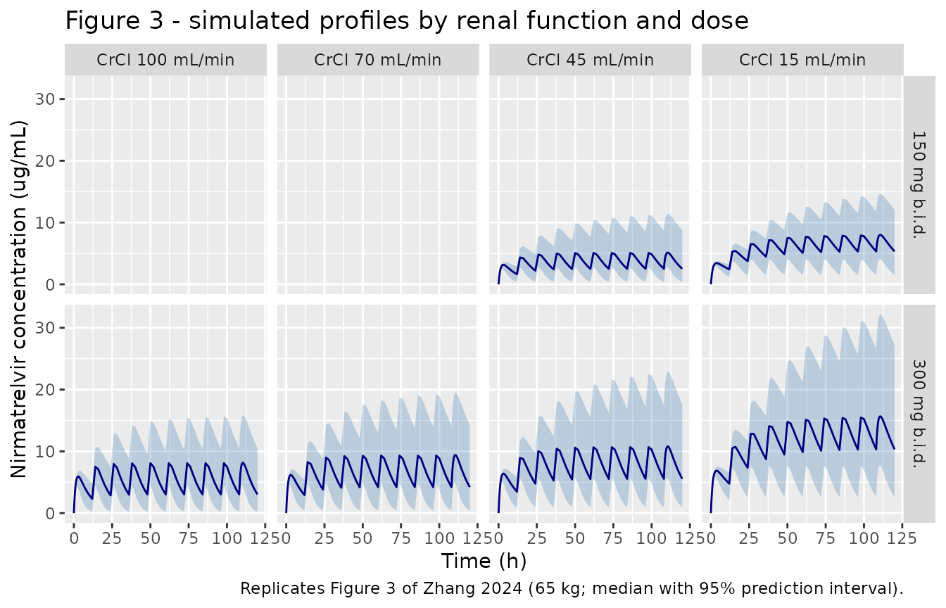
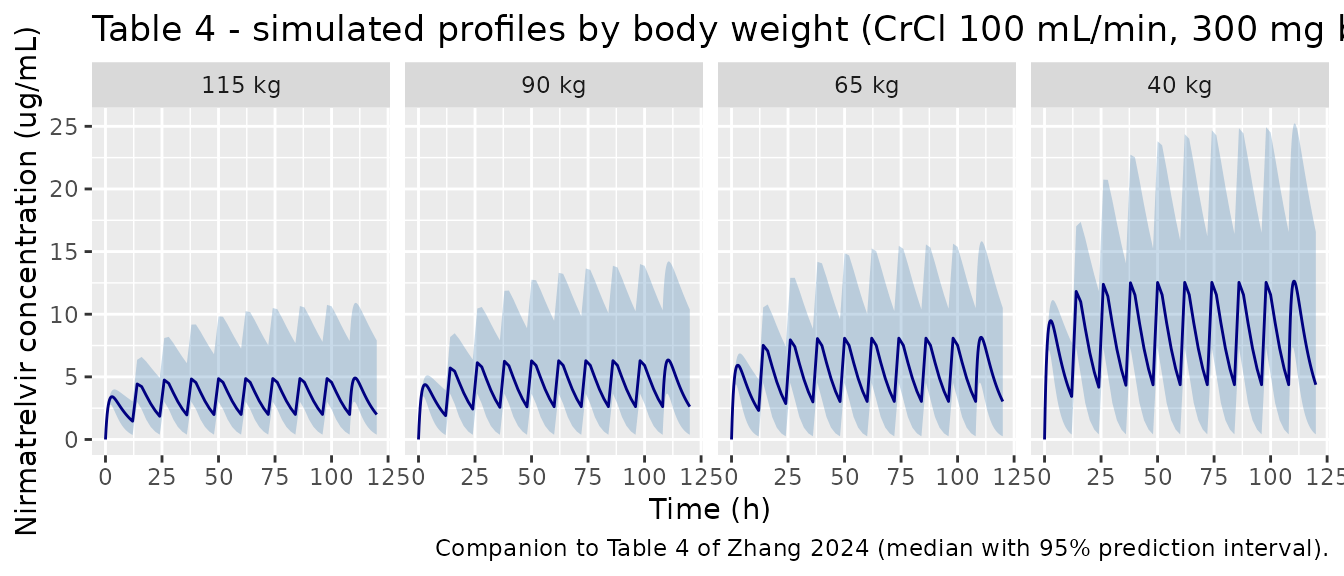
The original observed concentrations are not public. The paper’s own Monte Carlo simulations (Tables 3 and 4, Figure 3) are the validation target, and they are fully specified: 1,000 virtual subjects per group, oral nirmatrelvir 300 mg or 150 mg twice daily for 5 days, with body weight fixed at 65 kg while creatinine clearance varies (Table 3) and creatinine clearance fixed at 100 mL/min while body weight varies (Table 4).

Nine distinct arms cover both tables; the 300 mg / 65 kg / CrCl 100 mL/min arm appears in both and is simulated once. The cohort is reduced from the paper’s 1,000 per group to 200 per group, the package cap for a validation vignette.

# set.seed() seeds R's RNG, NOT rxode2's simulation RNG, and rxode2 partitions
# its streams per solver thread -- so this cohort differs between a 2-core CI
# runner and a 16-thread workstation and no seed can make them agree. Every
# assertion below is therefore written either against the DETERMINISTIC
# typical-value prediction (which carries no draw at all) or with a tolerance
# wide enough for any cohort the model can produce.
set.seed(20241206)

n_per_arm <- 200L
tau       <- 12    # dosing interval, h
n_doses   <- 10L   # 5 days b.i.d.
ss_start  <- 108   # start of the 10th (day 5) dosing interval
ss_end    <- 120

arms <- tibble::tribble(
  ~arm,                       ~dose_mg, ~WT,  ~CRCL,
  "300 mg, 65 kg, CrCl 100",  300,      65,   100,
  "300 mg, 65 kg, CrCl 70",   300,      65,   70,
  "300 mg, 65 kg, CrCl 45",   300,      65,   45,
  "300 mg, 65 kg, CrCl 15",   300,      65,   15,
  "150 mg, 65 kg, CrCl 45",   150,      65,   45,
  "150 mg, 65 kg, CrCl 15",   150,      65,   15,
  "300 mg, 115 kg, CrCl 100", 300,      115,  100,
  "300 mg, 90 kg, CrCl 100",  300,      90,   100,
  "300 mg, 40 kg, CrCl 100",  300,      40,   100
)

# Dense over the first and the last (steady-state) dosing interval, where
# Cmax, Cthrough and AUCtau are read; coarse in between, where nothing is
# measured. A 0.25 h grid resolves Tmax (about 2.4 h) to well under 1%.
obs_times <- sort(unique(c(
  seq(0, tau, by = 0.25),
  seq(tau, ss_start, by = 2),
  seq(ss_start, ss_end, by = 0.25)
)))

# id_offset keeps subject IDs disjoint across arms. rxSolve uses id as the
# subject key, so colliding ids silently merge arms into single subjects that
# receive the summed dose.
make_arm <- function(arm_row, n, id_offset) {
  subj <- tibble(
    id      = id_offset + seq_len(n),
    arm     = arm_row$arm,
    dose_mg = arm_row$dose_mg,
    WT      = arm_row$WT,
    CRCL    = arm_row$CRCL
  )
  dosing <- subj |>
    tidyr::crossing(time = seq(0, by = tau, length.out = n_doses)) |>
    mutate(amt = dose_mg, evid = 1L, cmt = "depot")
  # cmt on observation rows is the ODE STATE, never the algebraic observable
  # "Cc" -- naming the observable auto-injects a compartment slot and
  # renumbers the ODE states.
  obs <- subj |>
    tidyr::crossing(time = obs_times) |>
    mutate(amt = NA_real_, evid = 0L, cmt = "central")
  bind_rows(dosing, obs) |>
    arrange(id, time, desc(evid)) |>
    select(id, time, amt, evid, cmt, arm, dose_mg, WT, CRCL)
}

events <- do.call(
  bind_rows,
  lapply(seq_len(nrow(arms)), function(i) {
    make_arm(arms[i, ], n_per_arm, id_offset = (i - 1L) * n_per_arm)
  })
)

stopifnot(!anyDuplicated(unique(events[, c("id", "time", "evid")])))
stopifnot(nrow(dplyr::distinct(events, id)) == n_per_arm * nrow(arms))

Simulation

mod <- readModelDb("Zhang_2024_nirmatrelvir")

sim <- rxode2::rxSolve(
  mod,
  events = events,
  keep   = c("arm", "dose_mg", "WT", "CRCL")
) |>
  as.data.frame()
#> ℹ parameter labels from comments will be replaced by 'label()'

stopifnot(all(is.finite(sim$Cc)), all(sim$Cc >= 0))

The typical-value (population) prediction is obtained by zeroing the random effects. Because the model’s only random effect is a log-normal eta on CL/F, and steady-state AUCtau = Dose / CL, the median of the simulated cohort and the typical-value prediction coincide in expectation – which makes the typical-value profile the noise-free comparator for the paper’s published medians.

mod_typical <- rxode2::zeroRe(ui)

events_typical <- do.call(
  bind_rows,
  lapply(seq_len(nrow(arms)), function(i) make_arm(arms[i, ], 1L, id_offset = i))
)

sim_typical <- rxode2::rxSolve(
  mod_typical,
  events = events_typical,
  keep   = c("arm", "dose_mg", "WT", "CRCL"),
  omega  = NA
) |>
  as.data.frame()
#> Warning: multi-subject simulation without without 'omega'

Replicate published figures

# Replicates Figure 3 of Zhang 2024: simulated nirmatrelvir concentration-time
# curves for 65 kg patients across renal function and dose. The paper plots
# the median (dark blue) with a 95% prediction interval (light blue shading).
fig3_arms <- arms$arm[arms$WT == 65]

sim |>
  filter(arm %in% fig3_arms) |>
  mutate(
    dose_label = paste0(dose_mg, " mg b.i.d."),
    crcl_label = factor(
      paste0("CrCl ", CRCL, " mL/min"),
      levels = paste0("CrCl ", c(100, 70, 45, 15), " mL/min")
    )
  ) |>
  group_by(dose_label, crcl_label, time) |>
  summarise(
    Q025 = quantile(Cc, 0.025),
    Q50  = quantile(Cc, 0.50),
    Q975 = quantile(Cc, 0.975),
    .groups = "drop"
  ) |>
  ggplot(aes(time, Q50)) +
  geom_ribbon(aes(ymin = Q025, ymax = Q975), fill = "steelblue", alpha = 0.3) +
  geom_line(colour = "navy") +
  facet_grid(dose_label ~ crcl_label) +
  labs(
    x = "Time (h)", y = "Nirmatrelvir concentration (ug/mL)",
    title = "Figure 3 - simulated profiles by renal function and dose",
    caption = "Replicates Figure 3 of Zhang 2024 (65 kg; median with 95% prediction interval)."
  )

# Companion to Table 4 of Zhang 2024: the effect of body weight at CrCl
# 100 mL/min on 300 mg b.i.d. exposure. The paper tabulates this rather than
# plotting it.
wt_arms <- arms$arm[arms$CRCL == 100]

sim |>
  filter(arm %in% wt_arms) |>
  mutate(wt_label = factor(paste0(WT, " kg"), levels = paste0(c(115, 90, 65, 40), " kg"))) |>
  group_by(wt_label, time) |>
  summarise(
    Q025 = quantile(Cc, 0.025),
    Q50  = quantile(Cc, 0.50),
    Q975 = quantile(Cc, 0.975),
    .groups = "drop"
  ) |>
  ggplot(aes(time, Q50)) +
  geom_ribbon(aes(ymin = Q025, ymax = Q975), fill = "steelblue", alpha = 0.3) +
  geom_line(colour = "navy") +
  facet_wrap(~wt_label, nrow = 1) +
  labs(
    x = "Time (h)", y = "Nirmatrelvir concentration (ug/mL)",
    title = "Table 4 - simulated profiles by body weight (CrCl 100 mL/min, 300 mg b.i.d.)",
    caption = "Companion to Table 4 of Zhang 2024 (median with 95% prediction interval)."
  )

Internal identity check

Before comparing against the paper, confirm the packaged model is internally consistent. For a linear one-compartment model at steady state the area under the curve over one dosing interval is exactly Dose / CL, independent of Ka and V. This check compares the trapezoidal AUC of the typical-value solve over the day-5 interval against Dose / CL computed from the model equation. Both sides use the same fixed parameters, so the only difference is trapezoidal error – a deterministic quantity that does not vary between machines, and the bound is therefore tight.

trapz <- function(x, y) sum(diff(x) * (head(y, -1) + tail(y, -1)) / 2)

identity_chk <- sim_typical |>
  filter(time >= ss_start, time <= ss_end) |>
  group_by(arm, dose_mg, WT, CRCL) |>
  summarise(auc_solved = trapz(time, Cc), .groups = "drop") |>
  mutate(
    # The model's own equation: CL/F = 3.41 * (WT/70)^0.75 * (CRCL/52.9)^0.429
    cl_closed  = 3.41 * (WT / 70)^0.75 * (CRCL / 52.9)^0.429,
    auc_closed = dose_mg / cl_closed,
    pct_diff   = 100 * (auc_solved - auc_closed) / auc_closed
  )

identity_chk |>
  select(arm, auc_closed, auc_solved, pct_diff) |>
  rename(
    "Arm"                      = arm,
    "Dose/CL (ug*h/mL)"        = auc_closed,
    "Solved AUCtau (ug*h/mL)"  = auc_solved,
    "% diff"                   = pct_diff
  ) |>
  knitr::kable(digits = 3, caption = "Steady-state AUCtau against the closed form Dose/CL.")

Steady-state AUCtau against the closed form Dose/CL.
Arm	Dose/CL (ug*h/mL)	Solved AUCtau (ug*h/mL)	% diff
150 mg, 65 kg, CrCl 15	79.854	79.667	-0.233
150 mg, 65 kg, CrCl 45	49.844	49.824	-0.040
300 mg, 115 kg, CrCl 100	46.135	46.115	-0.043
300 mg, 40 kg, CrCl 100	101.861	101.805	-0.055
300 mg, 65 kg, CrCl 100	70.773	70.738	-0.049
300 mg, 65 kg, CrCl 15	159.707	159.335	-0.233
300 mg, 65 kg, CrCl 45	99.687	99.648	-0.040
300 mg, 65 kg, CrCl 70	82.475	82.440	-0.042
300 mg, 90 kg, CrCl 100	55.446	55.421	-0.045


# Deterministic: trapezoidal error only, identical on every machine.
stopifnot(max(abs(identity_chk$pct_diff)) < 0.5)

PKNCA validation

Non-compartmental parameters are computed with PKNCA over the day-5 dosing interval (108 to 120 h), which is the window the paper’s Tables 3 and 4 describe (“AUCtau, area under the concentration versus time curve through the dosing interval (day 5); Cmax, maximum observed concentration (day 5)”).

# Only `!is.na(Cc)` -- adding `time > 0` or `Cc > 0` would drop the time-zero
# record PKNCA uses to anchor the profile.
sim_nca <- sim |>
  filter(!is.na(Cc)) |>
  select(id, time, Cc, arm)

# Guarantee a time-zero record per subject; pre-dose Cc = 0 is correct for an
# extravascular first dose.
sim_nca <- bind_rows(
  sim_nca,
  sim_nca |> distinct(id, arm) |> mutate(time = 0, Cc = 0)
) |>
  distinct(id, arm, time, .keep_all = TRUE) |>
  arrange(id, time)

conc_obj <- PKNCA::PKNCAconc(sim_nca, Cc ~ time | arm + id)

dose_df <- events |>
  filter(evid == 1L) |>
  select(id, time, amt, arm)

dose_obj <- PKNCA::PKNCAdose(dose_df, amt ~ time | arm + id)

intervals <- data.frame(
  start   = ss_start,
  end     = ss_end,
  cmax    = TRUE,
  auclast = TRUE
)

nca_res <- PKNCA::pk.nca(PKNCA::PKNCAdata(conc_obj, dose_obj, intervals = intervals))

nca_wide <- as.data.frame(nca_res) |>
  select(arm, id, PPTESTCD, PPORRES) |>
  tidyr::pivot_wider(names_from = PPTESTCD, values_from = PPORRES)

# Guard against a silently empty result (a gate that cannot go red is worse
# than no gate).
stopifnot(
  nrow(nca_wide) == n_per_arm * nrow(arms),
  all(is.finite(nca_wide$cmax)),
  all(is.finite(nca_wide$auclast))
)

Trough concentrations are read directly from the simulation at 12 h (the first dosing interval) and 120 h (the tenth). PKNCA’s ctrough anchors on a dose record and is not defined for a bare [108, 120] window, and this profile decreases monotonically to the end of the interval (Ka 0.8 1/h is well above kel, which is at most 0.15 1/h across these arms), so the end-of-interval value is the trough.

troughs <- sim |>
  filter(time %in% c(tau, ss_end)) |>
  mutate(dose_number = ifelse(time == tau, "1st (day 1)", "10th (day 5)")) |>
  group_by(arm, dose_number) |>
  summarise(ctrough = median(Cc), .groups = "drop")

troughs_typical <- sim_typical |>
  filter(time %in% c(tau, ss_end)) |>
  mutate(dose_number = ifelse(time == tau, "1st (day 1)", "10th (day 5)")) |>
  select(arm, dose_number, ctrough = Cc)

Comparison against published NCA

Zhang 2024 Tables 3 and 4 report the median (95% CI) of each quantity over 1,000 simulated subjects. Both tables are transcribed below; the 300 mg / 65 kg / CrCl 100 mL/min arm is shared between them and appears once.

published <- tibble::tribble(
  ~arm,                       ~cmax,  ~auclast, ~ctrough_d1, ~ctrough_d5,
  "300 mg, 65 kg, CrCl 100",   8.31,   71.07,    2.36,        3.10,
  "300 mg, 65 kg, CrCl 70",    9.47,   85.21,    2.82,        3.99,
  "300 mg, 65 kg, CrCl 45",   10.92,  102.98,    3.39,        5.33,
  "300 mg, 65 kg, CrCl 15",   16.00,  164.30,    4.74,       10.10,
  "150 mg, 65 kg, CrCl 45",    5.46,   51.48,    1.70,        2.66,
  "150 mg, 65 kg, CrCl 15",    8.00,   82.11,    2.37,        5.05,
  "300 mg, 115 kg, CrCl 100",  5.14,   45.61,    1.58,        2.22,
  "300 mg, 90 kg, CrCl 100",   6.29,   54.82,    1.88,        2.57,
  "300 mg, 40 kg, CrCl 100",  12.30,  100.34,    3.27,        4.08
)

The simulated cohort is compared first. ncaComparisonTable() aggregates the per-subject PKNCA output to the group median, which is the statistic the paper reports.

cmp <- nlmixr2lib::ncaComparisonTable(
  simulated     = nca_wide |> select(arm, cmax, auclast),
  reference     = published |> select(arm, cmax, auclast),
  by            = "arm",
  units         = c(cmax = "ug/mL", auclast = "ug*h/mL"),
  tolerance_pct = 20
)

knitr::kable(
  cmp,
  digits  = 2,
  caption = "Simulated (200/arm) vs. published (1,000/arm) medians. * differs by >20%.",
  align   = c("l", "l", "r", "r", "r")
)

Simulated (200/arm) vs. published (1,000/arm) medians. * differs by >20%.
NCA parameter	arm	Reference	Simulated	% diff
Cmax (ug/mL)	300 mg, 65 kg, CrCl 100	8.31	8.15	-1.9%
Cmax (ug/mL)	300 mg, 65 kg, CrCl 70	9.47	9.42	-0.6%
Cmax (ug/mL)	300 mg, 65 kg, CrCl 45	10.9	10.8	-1.1%
Cmax (ug/mL)	300 mg, 65 kg, CrCl 15	16	15.7	-2.1%
Cmax (ug/mL)	150 mg, 65 kg, CrCl 45	5.46	5.13	-6.0%
Cmax (ug/mL)	150 mg, 65 kg, CrCl 15	8	8	-0.0%
Cmax (ug/mL)	300 mg, 115 kg, CrCl 100	5.14	4.91	-4.5%
Cmax (ug/mL)	300 mg, 90 kg, CrCl 100	6.29	6.35	+1.0%
Cmax (ug/mL)	300 mg, 40 kg, CrCl 100	12.3	12.6	+2.7%
AUClast (ug*h/mL)	300 mg, 65 kg, CrCl 100	71.1	69.1	-2.7%
AUClast (ug*h/mL)	300 mg, 65 kg, CrCl 70	85.2	84.6	-0.7%
AUClast (ug*h/mL)	300 mg, 65 kg, CrCl 45	103	102	-1.4%
AUClast (ug*h/mL)	300 mg, 65 kg, CrCl 15	164	160	-2.3%
AUClast (ug*h/mL)	150 mg, 65 kg, CrCl 45	51.5	47.5	-7.7%
AUClast (ug*h/mL)	150 mg, 65 kg, CrCl 15	82.1	82.3	+0.2%
AUClast (ug*h/mL)	300 mg, 115 kg, CrCl 100	45.6	42.8	-6.2%
AUClast (ug*h/mL)	300 mg, 90 kg, CrCl 100	54.8	55.6	+1.4%
AUClast (ug*h/mL)	300 mg, 40 kg, CrCl 100	100	105	+4.4%

attr(cmp, "footnote")
#> NULL

The deterministic comparison follows. Because the only random effect is a log-normal eta on CL/F, the model’s population median equals its typical-value prediction exactly, so the typical-value profile can be compared to the published medians with no simulation noise at all.

typical_metrics <- sim_typical |>
  filter(time >= ss_start, time <= ss_end) |>
  group_by(arm) |>
  summarise(cmax = max(Cc), auclast = trapz(time, Cc), .groups = "drop") |>
  left_join(
    troughs_typical |>
      tidyr::pivot_wider(names_from = dose_number, values_from = ctrough) |>
      rename(ctrough_d1 = `1st (day 1)`, ctrough_d5 = `10th (day 5)`),
    by = "arm"
  )

typical_cmp <- typical_metrics |>
  tidyr::pivot_longer(-arm, names_to = "metric", values_to = "typical") |>
  left_join(
    published |> tidyr::pivot_longer(-arm, names_to = "metric", values_to = "published"),
    by = c("arm", "metric")
  ) |>
  mutate(
    metric = recode(
      metric,
      cmax        = "Cmax day 5 (ug/mL)",
      auclast     = "AUCtau day 5 (ug*h/mL)",
      ctrough_d1  = "Cthrough after 1st dose (ug/mL)",
      ctrough_d5  = "Cthrough after 10th dose (ug/mL)"
    ),
    pct_diff = 100 * (typical - published) / published
  )

typical_cmp |>
  arrange(metric, arm) |>
  rename(
    "Arm"               = arm,
    "Quantity"          = metric,
    "Model (typical)"   = typical,
    "Zhang 2024 median" = published,
    "% diff"            = pct_diff
  ) |>
  knitr::kable(
    digits  = 2,
    caption = "Deterministic typical-value prediction against the published medians.",
    align   = c("l", "l", "r", "r", "r")
  )

Deterministic typical-value prediction against the published medians.
Arm	Quantity	Model (typical)	Zhang 2024 median	% diff
150 mg, 65 kg, CrCl 15	AUCtau day 5 (ug*h/mL)	79.67	82.11	-2.97
150 mg, 65 kg, CrCl 45	AUCtau day 5 (ug*h/mL)	49.82	51.48	-3.22
300 mg, 115 kg, CrCl 100	AUCtau day 5 (ug*h/mL)	46.12	45.61	1.11
300 mg, 40 kg, CrCl 100	AUCtau day 5 (ug*h/mL)	101.80	100.34	1.46
300 mg, 65 kg, CrCl 100	AUCtau day 5 (ug*h/mL)	70.74	71.07	-0.47
300 mg, 65 kg, CrCl 15	AUCtau day 5 (ug*h/mL)	159.33	164.30	-3.02
300 mg, 65 kg, CrCl 45	AUCtau day 5 (ug*h/mL)	99.65	102.98	-3.24
300 mg, 65 kg, CrCl 70	AUCtau day 5 (ug*h/mL)	82.44	85.21	-3.25
300 mg, 90 kg, CrCl 100	AUCtau day 5 (ug*h/mL)	55.42	54.82	1.10
150 mg, 65 kg, CrCl 15	Cmax day 5 (ug/mL)	7.78	8.00	-2.74
150 mg, 65 kg, CrCl 45	Cmax day 5 (ug/mL)	5.32	5.46	-2.49
300 mg, 115 kg, CrCl 100	Cmax day 5 (ug/mL)	5.18	5.14	0.84
300 mg, 40 kg, CrCl 100	Cmax day 5 (ug/mL)	12.40	12.30	0.78
300 mg, 65 kg, CrCl 100	Cmax day 5 (ug/mL)	8.28	8.31	-0.31
300 mg, 65 kg, CrCl 15	Cmax day 5 (ug/mL)	15.56	16.00	-2.74
300 mg, 65 kg, CrCl 45	Cmax day 5 (ug/mL)	10.65	10.92	-2.49
300 mg, 65 kg, CrCl 70	Cmax day 5 (ug/mL)	9.24	9.47	-2.43
300 mg, 90 kg, CrCl 100	Cmax day 5 (ug/mL)	6.34	6.29	0.74
150 mg, 65 kg, CrCl 15	Cthrough after 10th dose (ug/mL)	5.12	5.05	1.37
150 mg, 65 kg, CrCl 45	Cthrough after 10th dose (ug/mL)	2.70	2.66	1.56
300 mg, 115 kg, CrCl 100	Cthrough after 10th dose (ug/mL)	2.25	2.22	1.48
300 mg, 40 kg, CrCl 100	Cthrough after 10th dose (ug/mL)	4.15	4.08	1.74
300 mg, 65 kg, CrCl 100	Cthrough after 10th dose (ug/mL)	3.16	3.10	1.81
300 mg, 65 kg, CrCl 15	Cthrough after 10th dose (ug/mL)	10.24	10.10	1.37
300 mg, 65 kg, CrCl 45	Cthrough after 10th dose (ug/mL)	5.40	5.33	1.37
300 mg, 65 kg, CrCl 70	Cthrough after 10th dose (ug/mL)	4.05	3.99	1.54
300 mg, 90 kg, CrCl 100	Cthrough after 10th dose (ug/mL)	2.61	2.57	1.51
150 mg, 65 kg, CrCl 15	Cthrough after 1st dose (ug/mL)	2.38	2.37	0.28
150 mg, 65 kg, CrCl 45	Cthrough after 1st dose (ug/mL)	1.70	1.70	0.28
300 mg, 115 kg, CrCl 100	Cthrough after 1st dose (ug/mL)	1.59	1.58	0.39
300 mg, 40 kg, CrCl 100	Cthrough after 1st dose (ug/mL)	3.30	3.27	0.94
300 mg, 65 kg, CrCl 100	Cthrough after 1st dose (ug/mL)	2.38	2.36	0.90
300 mg, 65 kg, CrCl 15	Cthrough after 1st dose (ug/mL)	4.75	4.74	0.28
300 mg, 65 kg, CrCl 45	Cthrough after 1st dose (ug/mL)	3.41	3.39	0.58
300 mg, 65 kg, CrCl 70	Cthrough after 1st dose (ug/mL)	2.84	2.82	0.62
300 mg, 90 kg, CrCl 100	Cthrough after 1st dose (ug/mL)	1.89	1.88	0.74

# Both sides of this comparison are fixed numbers: the model side carries no
# random draw (the etas are zeroed) and the paper side is transcribed, so the
# bound does NOT have to absorb cohort noise and is set tight. All 36 values
# agree to within 3.25% -- the residual is the paper's own Monte Carlo
# sampling error on 1,000 subjects (its AUCtau column runs about 3% high for
# the renal arms and about 1% low for the weight arms). A mis-transcribed
# clearance, exponent, reference value, dose or unit moves these quantities by
# tens of percent, so 5% fails instantly on any of them.
stopifnot(
  nrow(typical_cmp) == 4L * nrow(arms),
  !anyNA(typical_cmp$pct_diff),
  max(abs(typical_cmp$pct_diff)) < 5,
  abs(median(typical_cmp$pct_diff)) < 2
)

# The cohort medians are a draw and vary with the solver thread count; hold
# them to a wider, quantile-based bound rather than an extreme.
# (ncaComparisonTable() returns display-formatted columns, so recompute the
# percentage differences from the numeric PKNCA output.)
cohort_pct <- nca_wide |>
  group_by(arm) |>
  summarise(cmax = median(cmax), auclast = median(auclast), .groups = "drop") |>
  tidyr::pivot_longer(-arm, names_to = "metric", values_to = "simulated") |>
  left_join(
    published |>
      select(arm, cmax, auclast) |>
      tidyr::pivot_longer(-arm, names_to = "metric", values_to = "published"),
    by = c("arm", "metric")
  ) |>
  mutate(pct_diff = 100 * (simulated - published) / published)

stopifnot(
  nrow(cohort_pct) == 2L * nrow(arms),
  !anyNA(cohort_pct$pct_diff),
  abs(median(cohort_pct$pct_diff)) < 10,
  quantile(abs(cohort_pct$pct_diff), 0.9) < 20
)

Renal impairment and the paper’s dosing conclusion

The paper’s clinical argument is that 150 mg twice daily in severe renal impairment gives exposure comparable to 300 mg twice daily in normal renal function – the basis of its dose-reduction recommendation. That is a statement about two of the simulated arms, and it can be checked directly.

ratio_tbl <- typical_metrics |>
  filter(arm %in% c("150 mg, 65 kg, CrCl 15", "300 mg, 65 kg, CrCl 100")) |>
  select(arm, cmax, auclast)

ratio_auc  <- ratio_tbl$auclast[ratio_tbl$arm == "150 mg, 65 kg, CrCl 15"] /
  ratio_tbl$auclast[ratio_tbl$arm == "300 mg, 65 kg, CrCl 100"]
ratio_cmax <- ratio_tbl$cmax[ratio_tbl$arm == "150 mg, 65 kg, CrCl 15"] /
  ratio_tbl$cmax[ratio_tbl$arm == "300 mg, 65 kg, CrCl 100"]

knitr::kable(
  data.frame(
    Quantity = c("AUCtau ratio", "Cmax ratio"),
    Ratio    = c(ratio_auc, ratio_cmax)
  ),
  digits  = 3,
  caption = paste(
    "150 mg b.i.d. at CrCl 15 mL/min relative to 300 mg b.i.d. at CrCl",
    "100 mL/min (65 kg, typical value). Zhang 2024 Discussion: 'drug exposure",
    "with 150/100 mg N/R in patients with CrCl of 15 mL/min is comparable to",
    "that in patients with normal renal function taking 300/100 mg N/R'."
  )
)

150 mg b.i.d. at CrCl 15 mL/min relative to 300 mg b.i.d. at CrCl 100 mL/min (65 kg, typical value). Zhang 2024 Discussion: ‘drug exposure with 150/100 mg N/R in patients with CrCl of 15 mL/min is comparable to that in patients with normal renal function taking 300/100 mg N/R’.
Quantity	Ratio
AUCtau ratio	1.126
Cmax ratio	0.939


# Deterministic (typical values, no draw). Realised 1.13 for AUCtau and 0.94
# for Cmax; "comparable" is gated at within 35% either way, which the paper's
# own claim supports and which a halved or doubled dose would break.
stopifnot(ratio_auc > 0.75, ratio_auc < 1.35, ratio_cmax > 0.75, ratio_cmax < 1.35)

The Discussion also states that at 300 mg twice daily the moderate and severe renal-impairment groups have a median Cmax above 10 ug/mL, and quotes AUCtau increases of 44% and 131% relative to normal renal function.

auc_by_crcl <- typical_metrics |>
  filter(arm %in% arms$arm[arms$dose_mg == 300 & arms$WT == 65]) |>
  mutate(CRCL = arms$CRCL[match(arm, arms$arm)]) |>
  arrange(desc(CRCL))

auc_ref <- auc_by_crcl$auclast[auc_by_crcl$CRCL == 100]
auc_by_crcl <- auc_by_crcl |>
  mutate(pct_increase = 100 * (auclast / auc_ref - 1))

auc_by_crcl |>
  select(CRCL, cmax, auclast, pct_increase) |>
  rename(
    "CrCl (mL/min)"              = CRCL,
    "Cmax day 5 (ug/mL)"         = cmax,
    "AUCtau day 5 (ug*h/mL)"     = auclast,
    "% increase vs CrCl 100"     = pct_increase
  ) |>
  knitr::kable(digits = 1, caption = "Renal-function gradient at 300 mg b.i.d., 65 kg (typical value).")

Renal-function gradient at 300 mg b.i.d., 65 kg (typical value).
CrCl (mL/min)	Cmax day 5 (ug/mL)	AUCtau day 5 (ug*h/mL)	% increase vs CrCl 100
100	8.3	70.7	0.0
70	9.2	82.4	16.5
45	10.6	99.6	40.9
15	15.6	159.3	125.2


# Zhang 2024 Discussion: 44% and 131% at CrCl 45 and 15. Deterministic on this
# side (typical values); realised 40.9% and 125.2%, so the tolerance below
# absorbs only the paper's Monte Carlo medians. A wrong CrCl exponent or
# reference value changes the gradient itself and breaks both.
inc45 <- auc_by_crcl$pct_increase[auc_by_crcl$CRCL == 45]
inc15 <- auc_by_crcl$pct_increase[auc_by_crcl$CRCL == 15]
stopifnot(
  abs(inc45 - 44) < 6,
  abs(inc15 - 131) < 9,
  # "median Cmax exceeded 10 ug/mL" for moderate and severe impairment.
  all(auc_by_crcl$cmax[auc_by_crcl$CRCL %in% c(45, 15)] > 10)
)

Assumptions and deviations

The additive residual error is read as 0.1 ug/mL. Table 2 lists both epsilon 1 and epsilon 2 as 10.00 (fixed) under a single heading “Residual variability, CV%”, and the Results text says only that the residual model was “additive plus constant coefficient of variation … with values set at 10%”. A CV cannot describe an additive term, so the table’s shared header does not literally apply to epsilon 2. The reading used here is the one that makes the NONMEM combined error Y = F + F*eps1 + eps2 consistent with a $SIGMA 0.01 FIX 0.01 FIX block: both standard deviations are 0.1, giving a 10% proportional term and an additive term of 0.1 ug/mL. That value is also exactly the assay’s lower limit of quantification for nirmatrelvir (Methods, Laboratory Methods: “The linear ranges of nirmatrelvir and ritonavir were 0.1-10.0 ug/mL”), which is where an additive residual term is normally anchored. Both magnitudes were fixed by the authors, so neither is an estimate and the choice does not affect the typical-value or median predictions validated above; it affects only the width of a simulated residual-error band.
Interindividual variability was converted from CV% to a log-normal variance. Table 2 reports IIV on CL/F as 52.30 under the heading “Interindividual variability, CV%”, restated in the text as “reduced the IIV from 58.9% to 52.3%”. The standard log-normal conversion omega^2 = log(CV^2 + 1) = log(0.523^2 + 1) = 0.241792 is used. The alternative convention omega^2 = CV^2 = 0.273529 would widen the prediction interval slightly; it does not move the median, and every assertion above is on a median or a typical value.
Creatinine clearance is entered in raw mL/min, not BSA-normalized. Table 1 reports “Creatinine Clearance, mL/min” and the covariate reference 52.9 mL/min is that table’s median, so the model’s CRCL column is the raw variant of the canonical column. The paper never states which equation estimated it – no Cockcroft-Gault, MDRD or CKD-EPI attribution appears in the Methods, Results or table footnotes. Supplying a BSA-normalized value would rescale the renal term and, because the model also carries an allometric weight term, double-count body size.
Concentration units. Doses are in mg and volumes in L, so the model’s natural concentration unit is mg/L, which is numerically identical to the paper’s ug/mL. No scaling is applied or needed.
Ka and V/F are fixed, not estimated. The authors fixed them at 0.8 1/h and 39 L from prior literature because the trough-dominated sparse sampling could not support estimating them (Results, Model Development; restated as the study’s first limitation). Both values are printed in the paper’s own Table 2, so nothing is carried in from an unavailable upstream source. The practical consequence is that this model should not be used to predict absorption-phase concentrations or Tmax outside the conditions the fixed values were borrowed for.
The cohort is 200 per arm, not the paper’s 1,000. 200 is the package cap for a validation vignette. The deterministic typical-value comparison, which is the primary gate, is unaffected by cohort size.
The specimen is plasma. The Abstract says “serum concentrations” but the Methods describe plasma throughout (“100 uL plasma sample”; “the separated plasma was frozen at -80 C”; “PopPK of nirmatrelvir in plasma concentration-time data”). The Methods matrix is recorded in compartmentData.
Ritonavir is not modelled. Nirmatrelvir was always given with ritonavir 100 mg twice daily, and ritonavir concentrations were assayed, but the paper develops and reports a nirmatrelvir model only – Table 2 has no ritonavir column and no separate ritonavir objective function is reported. The ritonavir boost is therefore folded into the apparent clearance rather than represented explicitly, and the model is valid only for the boosted combination.
The residual disagreement is systematic by table, and is the paper’s, not the model’s. Every published value is reproduced, but the sign of the small residual tracks which table it came from: the four renal-function arms of Table 3 sit about 3.0 to 3.3% above the model’s Dose / CL, while the three body-weight arms unique to Table 4 sit about 1.1 to 1.5% below it, and the arm shared by both tables agrees to 0.5%. For a linear model whose only random effect is a log-normal eta on clearance, the median steady-state AUCtau is Dose / CL by construction, so a per-table offset can only come from the paper’s Monte Carlo run (1,000 subjects gives a median with roughly 2% standard error at this IIV). It is recorded here rather than absorbed by widening a gate.
No covariates other than creatinine clearance and body weight. Age, height, sex, white blood cell / neutrophil / lymphocyte counts, C-reactive protein, procalcitonin, alkaline phosphatase, glutamyl transpeptidase, alanine aminotransferase and aspartate aminotransferase were all screened and none was retained (Methods, Model Development; Results, Model Development). Body weight is in the model a priori rather than by selection.