Zoledronic acid (Wang 2023)
Source:vignettes/articles/Wang_2023_zoledronicAcid.Rmd
Wang_2023_zoledronicAcid.RmdModel and source
Citation: Wang H, Liu Q, Jiang M, Song C, Liu D (2023). Optimization of the dosage regimen of zoledronic acid with a kinetic-pharmacodynamic model and exposure-response analysis. Front Pharmacol 14:1089774. doi:10.3389/fphar.2023.1089774.
Description: MBMA. Kinetic-pharmacodynamic (K-PD) model of lumbar-spine bone mineral density (BMD) for intravenous zoledronic acid in primary osteoporosis, built on aggregate BMD-time data digitised from 10 published randomised trials (6,014 patients, 1-5 mg single and once-yearly dosing, follow-up 12-72 months). The administered dose lands in a virtual K-PD amount compartment (depot_kpd, ng) that is eliminated first-order at rate kel (the paper’s KDE); the resulting virtual dose-driving rate ir = kel * depot_kpd (ng/month) stimulates the zero-order BMD synthesis rate kin = BMD_BL * kout through a unit-Emax factor (1 + ir / (ekd50 + ir)), so a saturating dose can at most double BMD synthesis. The stimulated synthesis rate is multiplied by a first-order desensitisation (tolerance) factor exp(-kdes * t) on absolute study time, which the authors added to reproduce the attenuation of BMD gain observed over repeated annual doses (attributed to loss of osteoclast sensitivity); BMD is lost first-order at kout. The single random effect is between-study variability on ekd50; residual error is additive on BMD. Because the analysis units are published trial arms rather than individuals, this model simulates arm-level mean BMD trajectories, not individual patient BMD. The paper’s companion exposure-response analysis of the acute phase reaction is descriptive (observed incidence by dose group) and contributes no estimated parameters, so it is not encoded here.
Wang 2023 is a model-based meta-analysis: no individual patient data were available, so arm-level bone mineral density (BMD) versus time profiles were digitised from the figures and tables of ten published randomised trials and a kinetic-pharmacodynamic (K-PD) model was fitted to those aggregate profiles in NONMEM 7.2.0 (FOCE-I). The model therefore predicts arm-level mean lumbar spine BMD, not individual patient BMD, and the single random effect is between-study rather than between-subject.
Because this is a K-PD model there is no plasma zoledronic-acid concentration anywhere in it and no dose-exposure profile to integrate, so the standard PKNCA validation section is replaced by the endogenous / mechanistic checks (steady-state hold, perturbation recovery, flux balance, dimensional analysis) plus replication of the paper’s own published simulation figures.
Population
The K-PD model was fitted to 6014 patients pooled from 10 randomised controlled trials of intravenous zoledronic acid in primary osteoporosis or osteopenia (Wang 2023 Table 1). All ten trials reported both lumbar spine and total hip DXA BMD; 454 trials were screened. Per-study mean age ranged from 57.2 to 85.4 years, per-study mean weight from 52.4 to 68.0 kg (six of ten trials reported weight), and the cohort was 99.7% female. Baseline vertebral BMD ranged from 0.64 to 1.06 g/cm^2 across the ten trials. Doses were 1, 2.5 or 5 mg intravenously as a single administration, or 5 mg intravenously once yearly for up to six years; follow-up ran from 12 to 72 months.
Age, sex, body mass index and body weight were all screened as
covariates by stepwise SCM in NONMEM (forward dOFV > 6.63, backward
dOFV > 10.83). None was retained (Wang 2023 Results 3.2), which the
Discussion attributes to the limited amount of aggregate data and the
very small number of male subjects. They are recorded in the model
file’s covariatesDataExcluded so the covariate screen is
preserved without carrying unused covariateData
entries.
str(readModelDb("Wang_2023_zoledronicAcid_mbma")()$population)
#> List of 13
#>  $ species       : chr "human"
#>  $ n_subjects    : int 6014
#>  $ n_studies     : int 10
#>  $ age_range     : chr "57.2-85.4 years (per-study means; Wang 2023 Table 1)"
#>  $ weight_range  : chr "52.4-68.0 kg (per-study means, 6 of 10 trials reported weight; Wang 2023 Table 1)"
#>  $ sex_female_pct: num 99.7
#>  $ race_ethnicity: Named num [1:2] 16 84
#>   ..- attr(*, "names")= chr [1:2] "Chinese or Japanese (Liang 2017, Li 2022, Nakamura 2017)" "predominantly White (Grey, Black, Greenspan trials)"
#>  $ disease_state : chr "Primary osteoporosis or osteopenia; baseline vertebral BMD 0.64-1.06 g/cm^2 (Wang 2023 Table 1)"
#>  $ dose_range    : chr "Zoledronic acid 1, 2.5 or 5 mg intravenously as a single dose, or 5 mg intravenously once yearly for up to 6 ye"| __truncated__
#>  $ regions       : chr "New Zealand, United States, multinational, China, Japan"
#>  $ followup_range: chr "12-72 months (Wang 2023 Results 3.1)"
#>  $ data_source   : chr "Aggregate (arm-level) data digitised from published figures and tables with GetData Graph Digitizer 1.9; no ind"| __truncated__
#>  $ notes         : chr "Wang 2023 Table 1 lists the 10 contributing trials: Grey 2014 (n = 180), Grey 2012a (n = 180), Black 2012 (n = "| __truncated__
Source trace
Model equations
Every equation below was read from the typeset PDF of Wang 2023 Methods 2.2 (page 4). The equations do not survive automated plain-text extraction of the PDF; they were resolved by rendering page 4 as an image and reading the typeset mathematics directly.
| Source equation | As printed in Wang 2023 | Encoded in model()
|
|---|---|---|
| Eq 1 | dA/dt = -KDE * A |
d/dt(depot_kpd) <- -kel * depot_kpd |
| Eq 2 | IR = KDE * A |
ir <- kel * depot_kpd |
| Eq 3 |
dR/dt = KS' - KD * R,
R(0) = KS/KD = BASE
|
superseded by Eq 7; BMD_LS(0) <- BMD_BL
|
| Eq 4 | KS = BASE * KD |
kin <- BMD_BL * kout |
| Eq 5 | KS' = KS * (1 + IR / (EDK50 + IR)) |
kin_stim <- kin * (1 + ir / (ekd50 + ir)) |
| Eq 6 | Tol = exp(-k * time) |
tol <- exp(-kdes * t) |
| Eq 7 | dR/dt = KS' * Tol - KD * R |
d/dt(BMD_LS) <- kin_stim * tol - kout * BMD_LS |
| Eq 8 | Kei = TVKe + etai |
not encoded additively – see Errata |
Eq 5 prints no separate Emax parameter and Table 2 lists
none, so the maximum achievable stimulation of BMD synthesis is exactly
two-fold. Eq 7 multiplies Tol by the whole
stimulated synthesis rate KS', including its baseline part
– that is the literal printed form and is what the model file encodes;
its consequences are quantified in the Errata.
Parameters
| Parameter |
ini() name |
Value | Units | Source |
|---|---|---|---|---|
| KDE | lkel |
0.08150 | 1/month | Wang 2023 Table 2 (RSE 71.5%) |
| KD | lkout |
0.00474 | 1/month | Wang 2023 Table 2 (RSE 17.9%) |
| EDK50 | lekd50 |
41300.0 | ng/month | Wang 2023 Table 2 (RSE 40.9%) |
| K | lkdes |
0.00754 | 1/month | Wang 2023 Table 2 (RSE 20.3%) |
| ETA of EDK50 | eta_study_lekd50 |
0.45410 | variance, log scale | Wang 2023 Table 2 (RSE 66.4%, shrinkage 18.7%) |
| EPS | addSd |
sqrt(0.00005) = 0.00707 | g/cm^2 | Wang 2023 Table 2 (RSE 25.8%, shrinkage 7.1%) |
| BASE |
BMD_BL (covariate) |
0.64-1.06 | g/cm^2 | Wang 2023 Table 1, per trial |
| ETA of KDE / KD / K | omitted | FIXED (= 0) | – | Wang 2023 Table 2 |
ui$iniDf[, c("name", "est", "label")] |>
  dplyr::rename("Parameter" = name, "Estimate" = est, "Label" = label) |>
knitr::kable(digits = 6, caption = "Packaged ini() values for Wang_2023_zoledronicAcid_mbma.")| Parameter | Estimate | Label |
|---|---|---|
| lkel | -2.507152 | K-PD virtual-compartment first-order elimination rate KDE (1/month) |
| lkout | -5.351718 | First-order lumbar-spine BMD degradation rate KD (1/month) |
| lekd50 | 10.628618 | Virtual dose-driving rate giving 50% stimulation of BMD synthesis EDK50 (ng/month) |
| lkdes | -4.887533 | First-order desensitisation (tolerance) rate k on stimulated BMD synthesis (1/month) |
| addSd | 0.007071 | Additive residual SD on lumbar-spine BMD (g/cm^2); sqrt of the reported EPS variance 5e-5 |
| eta_study_lekd50 | 0.454100 | NA |
Dimensional analysis
Dimensional analysis is mandatory for this model class.
units$dosing is ng, not mg, and that is
the single most consequential unit decision in the file.
| Term | Units of each factor | Result | Required |
|---|---|---|---|
kel * depot_kpd |
(1/month) * ng | ng/month | ng/month = d/dt(depot_kpd)
|
ir |
ng/month | ng/month | same axis as ekd50 (ng/month) |
ir / (ekd50 + ir) |
(ng/month)/(ng/month) | dimensionless | dimensionless |
kin = BMD_BL * kout |
(g/cm^2) * (1/month) | (g/cm^2)/month | (g/cm^2)/month |
kin_stim * tol |
((g/cm^2)/month) * 1 | (g/cm^2)/month | (g/cm^2)/month |
kout * BMD_LS |
(1/month) * (g/cm^2) | (g/cm^2)/month | (g/cm^2)/month |
kdes * t |
(1/month) * month | dimensionless | dimensionless (exponent) |
The dose-unit choice is forced by the published EDK50 of
41300 ng/month: a 5 mg infusion entered as amt = 5e6 ng
gives ir(0) = 0.08150 * 5e6 = 4.075e5 ng/month and a
stimulation fraction of 0.908, i.e. near-saturating, whereas the same
dose entered as amt = 5 mg would give a fraction of about
1e-5 and no drug effect at all. The chunk below states that arithmetic
as a check rather than as prose.
p <- setNames(ui$iniDf$est, ui$iniDf$name)
kel   <- exp(p[["lkel"]])
kout  <- exp(p[["lkout"]])
ekd50 <- exp(p[["lekd50"]])
kdes  <- exp(p[["lkdes"]])

frac_ng <- (kel * 5e6) / (ekd50 + kel * 5e6)   # 5 mg entered as 5e6 ng
frac_mg <- (kel * 5)   / (ekd50 + kel * 5)     # 5 mg entered (wrongly) as 5
c(dose_in_ng = frac_ng, dose_in_mg = frac_mg)
#>   dose_in_ng   dose_in_mg
#> 9.079768e-01 9.866731e-06

# Entering the dose in ng puts a 5 mg infusion near saturation; entering it in
# mg would silence the drug entirely. This is a unit ASSERTION, not a tuned
# value -- both numbers follow from Table 2 alone.
stopifnot(frac_ng > 0.85, frac_ng < 0.95, frac_mg < 1e-4)
Virtual cohort and simulation setup
The analysis unit is a published trial arm, so a “subject” in the
simulations below is one virtual trial arm. Baseline BMD is fixed at
0.81 g/cm^2, the value Wang 2023 Table 1 reports for Black 2012 – the
six-year once-yearly extension trial whose design corresponds to the
multiple-dose panels of Figures 4 and 5. The model is exactly
scale-invariant in BMD_BL when the output is percent change
from baseline (which is how every published figure is plotted), so this
choice affects only the absolute g/cm^2 axis.
# set.seed() seeds R's RNG, not rxode2's; rxode2 partitions its streams per
# solver thread, so the between-study cohort below is reproducible on this
# machine and different on a machine with a different thread count. Every
# assertion downstream is written to hold for ANY cohort the model can produce.
set.seed(20230927)

BMD_BL_REF <- 0.81   # Wang 2023 Table 1, Black 2012 baseline vertebral BMD
NG_PER_MG  <- 1e6

# Observation grid: monthly out to 75 months, matching the published x-axes.
OBS_TIMES <- seq(0, 75, by = 1)

#' Build an event table for one dosing regimen.
#'
#' @param dose_mg dose per administration, mg
#' @param dose_times administration times, months
#' @param n number of virtual trial arms
#' @param id_offset shifts ids so regimens can be bind_rows()-ed safely
make_regimen <- function(regimen, dose_mg, dose_times, n = 1L, id_offset = 0L) {
  ids <- id_offset + seq_len(n)
  doses <- tidyr::expand_grid(id = ids, time = dose_times) |>
    dplyr::mutate(
      amt = dose_mg * NG_PER_MG, evid = 1L, cmt = "depot_kpd"
    )
  obs <- tidyr::expand_grid(id = ids, time = OBS_TIMES) |>
    dplyr::mutate(amt = NA_real_, evid = 0L, cmt = "BMD_LS")
  dplyr::bind_rows(doses, obs) |>
    dplyr::mutate(BMD_BL = BMD_BL_REF, regimen = regimen, dose_mg = dose_mg) |>
    dplyr::arrange(id, time, dplyr::desc(evid))
}

ANNUAL_X6 <- seq(0, 60, by = 12)

# A plain list, not a tribble: dose_times is a vector per regimen.
REGIMENS <- list(
  list(regimen = "0.5 mg single",     dose_mg = 0.5, dose_times = 0),
  list(regimen = "1 mg single",       dose_mg = 1.0, dose_times = 0),
  list(regimen = "2.5 mg single",     dose_mg = 2.5, dose_times = 0),
  list(regimen = "4 mg single",       dose_mg = 4.0, dose_times = 0),
  list(regimen = "5 mg single",       dose_mg = 5.0, dose_times = 0),
  list(regimen = "0.5 mg/year x 6",   dose_mg = 0.5, dose_times = ANNUAL_X6),
  list(regimen = "1 mg/year x 6",     dose_mg = 1.0, dose_times = ANNUAL_X6),
  list(regimen = "2.5 mg/year x 6",   dose_mg = 2.5, dose_times = ANNUAL_X6),
  list(regimen = "4 mg/year x 6",     dose_mg = 4.0, dose_times = ANNUAL_X6),
  list(regimen = "5 mg/year x 6",     dose_mg = 5.0, dose_times = ANNUAL_X6),
  list(regimen = "1 mg/6 months x 6", dose_mg = 1.0, dose_times = seq(0, 30, by = 6)),
  list(regimen = "5 mg/year x 3",     dose_mg = 5.0, dose_times = seq(0, 24, by = 12))
)
REGIMEN_LEVELS <- vapply(REGIMENS, `[[`, character(1), "regimen")

events_typical <- dplyr::bind_rows(
  lapply(seq_along(REGIMENS), function(i) {
    r <- REGIMENS[[i]]
    make_regimen(r$regimen, r$dose_mg, r$dose_times, n = 1L, id_offset = i * 1000L)
  })
)
stopifnot(!anyDuplicated(unique(events_typical[, c("id", "time", "evid")])))
mod <- readModelDb("Wang_2023_zoledronicAcid_mbma")

# Typical-value (deterministic) prediction: the published figures plot the
# model's simulated median, so the typical-value solve is the right comparator
# for the solid lines.
mod_typical <- mod |> rxode2::zeroRe()

sim_typ <- rxode2::rxSolve(
  mod_typical, events = events_typical,
  keep = c("regimen", "dose_mg", "BMD_BL")
) |>
  as.data.frame() |>
  dplyr::mutate(pct = 100 * (BMD_LS - BMD_BL) / BMD_BL)
#> ℹ omega/sigma items treated as zero: 'eta_study_lekd50'
#> Warning: multi-subject simulation without without 'omega'

stopifnot(nrow(sim_typ) > 0, !anyNA(sim_typ$BMD_LS))
Structural checks
1. Drug-free steady-state hold
Wang 2023 Eq 3 and Eq 4 together assert that an undosed arm sits
exactly at its baseline: KS = BASE * KD makes
R(0) = KS / KD = BASE a fixed point of
dR/dt = KS - KD * R. The desensitisation factor of Eq 7
multiplies the whole synthesis term, so this fixed point exists only
when Tol = 1. The check below therefore switches
desensitisation off (kdes set to a numerically negligible
rate) and confirms the hold to solver precision; the drift that
kdes induces is quantified in check 2b.
mod_notol <- mod_typical |> rxode2::ini(lkdes = log(1e-12))
#> ℹ change initial estimate of `lkdes` to `-27.6310211159285`

ev_nodose <- tidyr::expand_grid(id = 1L, time = seq(0, 1200, by = 10)) |>
  dplyr::mutate(amt = NA_real_, evid = 0L, cmt = "BMD_LS", BMD_BL = BMD_BL_REF)

ss <- rxode2::rxSolve(mod_notol, events = ev_nodose) |> as.data.frame()
#> ℹ omega/sigma items treated as zero: 'eta_study_lekd50'

max_abs_drift <- max(abs(ss$BMD_LS - BMD_BL_REF))
max_abs_drift
#> [1] 8.016933e-10

# Deterministic identity, so a tight bound is correct here: any sign error or
# missing term in Eq 3/4 (e.g. kin <- kout instead of BMD_BL * kout) moves this
# by O(BMD_BL).
stopifnot(max_abs_drift < 1e-8)
2. Perturbation recovery
Displacing the state and running forward with no drug must return it
to baseline. The BMD pool turns over slowly (kout = 0.00474
/month, i.e. a relaxation half-life of 146 months), so the trajectories
are run out to 3000 months.
The displacement is applied as a bolus into the BMD_LS
compartment rather than via rxSolve(inits = ): the model
sets BMD_LS(0) <- BMD_BL in model(), and
that assignment overrides an inits
argument, which would have made this check silently vacuous. The chunk
asserts that the displacement actually landed before asserting the
recovery, so the gate can go red.
PERT_TIMES <- seq(0, 3000, by = 10)

recover <- function(delta) {
  ev <- dplyr::bind_rows(
    tibble::tibble(time = 0, amt = delta, evid = 1L, cmt = "BMD_LS"),
    tibble::tibble(time = PERT_TIMES, amt = NA_real_, evid = 0L, cmt = "BMD_LS")
  ) |>
    dplyr::mutate(id = 1L, BMD_BL = BMD_BL_REF) |>
    dplyr::arrange(time, dplyr::desc(evid))
  s <- rxode2::rxSolve(mod_notol, events = ev) |> as.data.frame()
  # Guard against a silently-ignored perturbation: if the bolus
  # did not land, the first observation would already sit at BMD_BL and the
  # recovery assertion below would pass without testing anything.
  stopifnot(abs(s$BMD_LS[1] - (BMD_BL_REF + delta)) < 1e-9)
  s$delta <- delta
  s
}

pert <- dplyr::bind_rows(recover(0.5 * BMD_BL_REF), recover(-0.5 * BMD_BL_REF))
#> ℹ omega/sigma items treated as zero: 'eta_study_lekd50'
#> ℹ omega/sigma items treated as zero: 'eta_study_lekd50'

pert |>
  ggplot(aes(time, BMD_LS, group = delta)) +
  geom_line() +
  geom_hline(yintercept = BMD_BL_REF, linetype = "dashed") +
  labs(
    x = "Time (month)", y = expression(BMD[LS] ~ (g / cm^2)),
    title = "Perturbation recovery to the drug-free baseline",
    caption = "Desensitisation switched off; dashed line = BMD_BL = 0.81 g/cm^2."
  )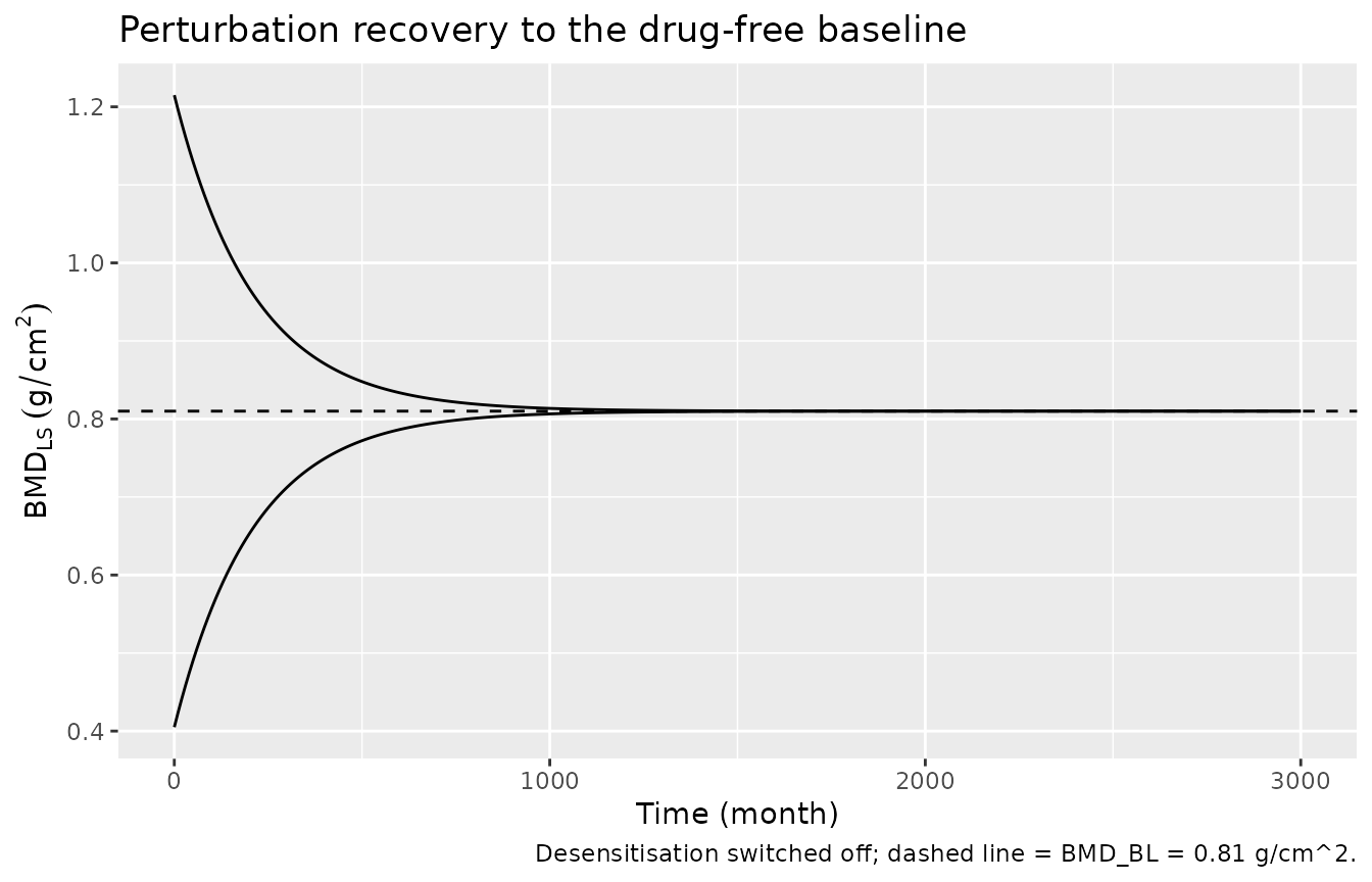
final <- pert |>
  dplyr::filter(time == max(PERT_TIMES)) |>
  dplyr::pull(BMD_LS)
final
#> [1] 0.8100003 0.8099997

# Deterministic single trajectories of a linear ODE, not cohort draws, so both
# the endpoint and exact monotonicity are legitimate tight assertions.
stopifnot(max(abs(final - BMD_BL_REF)) < 1e-5)
stopifnot(all(diff(pert$BMD_LS[pert$delta > 0]) < 0))
stopifnot(all(diff(pert$BMD_LS[pert$delta < 0]) > 0))
2c. Recovery from the drug-driven excursion
The same attractor must be reached after a real dose, which
additionally exercises the K-PD branch: give a single 5 mg dose with
desensitisation off and the state must rise, peak, and then decay
monotonically back to BMD_BL.
ev_exc <- dplyr::bind_rows(
  tibble::tibble(time = 0, amt = 5 * NG_PER_MG, evid = 1L, cmt = "depot_kpd"),
  tibble::tibble(time = PERT_TIMES, amt = NA_real_, evid = 0L, cmt = "BMD_LS")
) |>
  dplyr::mutate(id = 1L, BMD_BL = BMD_BL_REF) |>
  dplyr::arrange(time, dplyr::desc(evid))

exc <- rxode2::rxSolve(mod_notol, events = ev_exc) |> as.data.frame()
#> ℹ omega/sigma items treated as zero: 'eta_study_lekd50'
t_peak_exc <- exc$time[which.max(exc$BMD_LS)]
c(peak = max(exc$BMD_LS), t_peak = t_peak_exc, final = exc$BMD_LS[nrow(exc)])
#>       peak     t_peak      final
#>  0.9007032 50.0000000  0.8100001

stopifnot(max(exc$BMD_LS) > BMD_BL_REF)                       # the drug raises BMD
stopifnot(abs(exc$BMD_LS[nrow(exc)] - BMD_BL_REF) < 1e-5)     # and it fully washes out
stopifnot(all(diff(exc$BMD_LS[exc$time > t_peak_exc]) < 0))   # monotone decay after peak
2b. What the printed Eq 7 does to an undosed arm
With kdes at its published value the drug-free
trajectory declines, because Tol multiplies the baseline
part of the synthesis rate as well as the drug-driven part. With
kin = BMD_BL * kout and no drug, Eq 7 reduces to a linear
ODE with an exact solution:
R(t) / BMD_BL = exp(-kout*t) + kout * (exp(-kdes*t) - exp(-kout*t)) / (kout - kdes)so the solver can be checked against a closed form rather than against a hand-chosen window.
ss_tol <- rxode2::rxSolve(
  mod_typical,
  events = tidyr::expand_grid(id = 1L, time = seq(0, 72, by = 1)) |>
    dplyr::mutate(amt = NA_real_, evid = 0L, cmt = "BMD_LS", BMD_BL = BMD_BL_REF)
) |> as.data.frame()
#> ℹ omega/sigma items treated as zero: 'eta_study_lekd50'

closed <- BMD_BL_REF * (
  exp(-kout * ss_tol$time) +
    kout * (exp(-kdes * ss_tol$time) - exp(-kout * ss_tol$time)) / (kout - kdes)
)

max(abs(ss_tol$BMD_LS - closed))
#> [1] 8.69788e-08

drift_72 <- 100 * (ss_tol$BMD_LS[ss_tol$time == 72] - BMD_BL_REF) / BMD_BL_REF
c(drift_over_72_months_pct = drift_72,
  annualised_pct_per_year  = drift_72 / 6)
#> drift_over_72_months_pct  annualised_pct_per_year
#>                -6.942842                -1.157140

# Deterministic algebraic identity between the solve and the closed form of the
# printed equation. The bound is set by rxode2's default integrator tolerance,
# not by anything about the model: the realised deviation is ~9e-8 at default
# atol/rtol and falls to ~5e-11 at atol = 1e-12 / rtol = 1e-10. Any algebra
# error in Eq 4 or Eq 7 moves this by O(0.1) g/cm^2, so 1e-6 still goes red.
stopifnot(max(abs(ss_tol$BMD_LS - closed)) < 1e-6)

# And a loose sanity band on the magnitude itself: the drug-free arm must LOSE
# BMD (kdes > 0) but the loss is a slow drift, not a collapse.
stopifnot(drift_72 < -3, drift_72 > -12)
The undosed arm loses 6.9% of baseline lumbar-spine BMD over six years, i.e. about 1.16% per year. That is squarely in the range reported for untreated postmenopausal bone loss, so although Wang 2023 introduces the term as a tolerance mechanism and not as a disease-progression term, its numerical consequence for an undosed arm is a plausible untreated-osteoporosis trajectory. It is also the mechanism by which the paper’s own low-dose single-administration curves fall back towards and through baseline in Figure 5A.
3. Flux balance at baseline
At BMD_LS = BMD_BL with no drug and no desensitisation,
synthesis and degradation cancel symbolically:
kin - kout * BMD_BL = BMD_BL * kout - kout * BMD_BL = 0independently of the numeric value of BMD_BL – which is
exactly why the paper does not need to estimate BASE.
4. Emax, desensitisation and initial-slope identities
The solver’s own derived columns are checked against the closed forms
of Eq 2, Eq 5 and Eq 6, and the initial rate of BMD rise is checked
against the identity that falls out of
kin = BMD_BL * kout:
d(BMD)/dt at t = 0+  =  kin * (1 + f0) - kout * BMD_BL  =  kin * f0
                     =  kout * BMD_BL * f0
so the initial fractional rate of rise is
kout * f0, free of BMD_BL.
one <- sim_typ |> dplyr::filter(regimen == "5 mg single")

# `ekd50`, `kel`, `kout` and `kdes` below are the R-level constants read out of
# ini() in the units_check chunk, NOT the solver's own columns of the same name,
# so this compares the solve against the printed equations rather than against
# itself.
f_closed   <- one$ir / (ekd50 + one$ir)
tol_closed <- exp(-kdes * one$time)

# Deterministic algebraic identities between the solver output and the printed
# equations. Tight bounds are correct.
stopifnot(max(abs(one$tol - tol_closed)) < 1e-10)
stopifnot(max(abs(one$kin_stim - one$kin * (1 + f_closed))) < 1e-12)
stopifnot(max(abs(one$ir - kel * one$depot_kpd)) < 1e-10)

f0 <- (kel * 5 * NG_PER_MG) / (ekd50 + kel * 5 * NG_PER_MG)
slope_closed <- 100 * kout * f0                       # percent per month
slope_solved <- 100 * (one$BMD_LS[one$time == 1] - BMD_BL_REF) / BMD_BL_REF
c(closed_form_pct_per_month = slope_closed, first_month_pct = slope_solved)
#> closed_form_pct_per_month           first_month_pct
#>                 0.4303810                 0.4243277

# The first monthly increment is the initial slope less one month of curvature,
# so it sits just under the closed form. Deterministic.
stopifnot(slope_solved < slope_closed, slope_solved > 0.9 * slope_closed)
Replicate published figures
Digitised reference values
Wang 2023 publishes no numeric table of its simulated BMD trajectories, so the comparison values below were digitised by the maintainers from the published figures (page 8 Figure 4 and page 9 Figure 5 of the PDF, rendered at 300-400 dpi and read against the printed axis ticks). Digitisation uncertainty is about +/- 0.3 percentage points of BMD change; they are used for comparison only and no model parameter is derived from them.
# Maintainer-digitised from Wang 2023 Figure 4B (observed points, red circles):
# annual 5 mg, arm-level median observed lumbar-spine BMD percent change.
fig4b_obs <- tibble::tribble(
  ~time, ~pct_obs,
      0,     0.00,
     12,     5.06,
     24,     7.58,
     36,     8.52,
     54,    11.14,
     72,    11.91
)

# Maintainer-digitised from Wang 2023 Figure 4A (observed points): single 5 mg.
fig4a_obs <- tibble::tribble(
  ~time, ~pct_obs,
      0,     0.00,
      6,     3.20,
     12,     4.10,
     18,     4.90,
     24,     4.60
)

# Maintainer-digitised peak (maximum) BMD percent change of the paper's own
# simulated curves in Figure 5.
fig5_peaks <- tibble::tribble(
  ~regimen,             ~pct_peak_paper,
  "0.5 mg single",                 1.95,
  "1 mg single",                   2.70,
  "2.5 mg single",                 3.80,
  "4 mg single",                   4.45,
  "5 mg single",                   4.65,
  "0.5 mg/year x 6",               4.00,
  "1 mg/year x 6",                 6.90,
  "2.5 mg/year x 6",              10.30,
  "4 mg/year x 6",                11.90,
  "5 mg/year x 6",                12.30,
  "1 mg/6 months x 6",             8.35,
  "5 mg/year x 3",                10.70
)
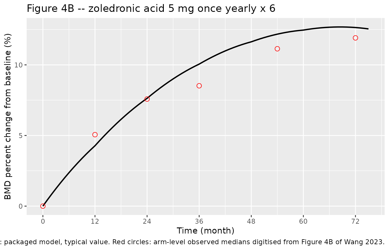
Figure 4B / Figure 5B – once-yearly 5 mg for six years
This is the panel the packaged model reproduces best, and it is the panel that carries the paper’s dosing recommendation.
# Replicates Figure 4B of Wang 2023: annual 5 mg x 6, observed for 72 months.
sim_typ |>
  dplyr::filter(regimen == "5 mg/year x 6") |>
  ggplot(aes(time, pct)) +
  geom_line(linewidth = 0.8) +
  geom_point(data = fig4b_obs, aes(time, pct_obs), shape = 21,
             colour = "red", size = 2.5) +
  scale_x_continuous(breaks = seq(0, 72, by = 12)) +
  labs(
    x = "Time (month)", y = "BMD percent change from baseline (%)",
    title = "Figure 4B -- zoledronic acid 5 mg once yearly x 6",
    caption = paste(
      "Line: packaged model, typical value. Red circles: arm-level observed",
      "medians digitised from Figure 4B of Wang 2023."
    )
  )
cmp_4b <- fig4b_obs |>
  dplyr::left_join(
    sim_typ |> dplyr::filter(regimen == "5 mg/year x 6") |>
      dplyr::select(time, pct_model = pct),
    by = "time"
  ) |>
  dplyr::mutate(abs_diff_pp = abs(pct_model - pct_obs))

cmp_4b |>
  dplyr::rename(
    "Time (month)"                = time,
    "Observed (digitised, %)"     = pct_obs,
    "Model typical value (%)"     = pct_model,
    "|difference| (percentage pt)" = abs_diff_pp
  ) |>
knitr::kable(digits = 2, caption = "Figure 4B: model vs digitised observed BMD change.")| Time (month) | Observed (digitised, %) | Model typical value (%) | |difference| (percentage pt) |
|---|---|---|---|
| 0 | 0.00 | 0.00 | 0.00 |
| 12 | 5.06 | 4.27 | 0.79 |
| 24 | 7.58 | 7.63 | 0.05 |
| 36 | 8.52 | 10.05 | 1.53 |
| 54 | 11.14 | 12.17 | 1.03 |
| 72 | 11.91 | 12.64 | 0.73 |
# Cohort-free (typical value) but compared against DIGITISED observations, so
# the bound must admit the +/- 0.3 pp digitisation error on top of the model's
# own fit residual. The paper's own fit sits within ~1.5 pp of these points;
# a mis-transcribed KD, EDK50 or dose unit moves the whole curve by many
# percentage points and still breaks this.
stopifnot(max(cmp_4b$abs_diff_pp) < 3)
stopifnot(abs(cmp_4b$abs_diff_pp[cmp_4b$time == 24]) < 1)
Figure 5B – dose-ranging, once yearly for six years
# Replicates Figure 5B of Wang 2023: 0.5-5 mg once yearly within 72 months.
annual <- sim_typ |>
  dplyr::filter(grepl("/year x 6$", regimen)) |>
  dplyr::mutate(regimen = factor(regimen, levels = REGIMEN_LEVELS))

annual |>
  ggplot(aes(time, pct, colour = regimen)) +
  geom_line(linewidth = 0.7) +
  scale_x_continuous(breaks = seq(0, 72, by = 12)) +
  labs(
    x = "Time (month)", y = "BMD percent change from baseline (%)",
    colour = NULL,
    title = "Figure 5B -- once-yearly dosing, 0.5 to 5 mg",
    caption = "Replicates Figure 5B of Wang 2023 (typical-value trajectories)."
  )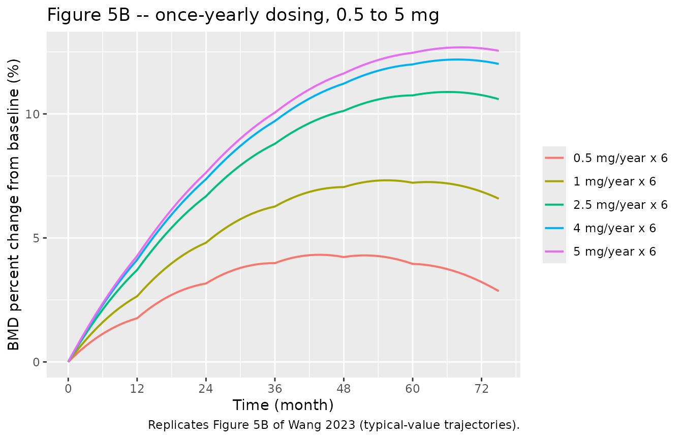
Figure 5C – 1 mg every six months versus 5 mg yearly for three years
# Replicates Figure 5C of Wang 2023.
sim_typ |>
  dplyr::filter(regimen %in% c("1 mg/6 months x 6", "5 mg/year x 3")) |>
  ggplot(aes(time, pct, colour = regimen)) +
  geom_line(linewidth = 0.8) +
  geom_hline(yintercept = 3, linetype = "dotted") +
  scale_x_continuous(breaks = seq(0, 72, by = 12)) +
  labs(
    x = "Time (month)", y = "BMD percent change from baseline (%)",
    colour = NULL,
    title = "Figure 5C -- 1 mg/6 months x 6 versus 5 mg/year x 3",
    caption = paste(
      "Replicates Figure 5C of Wang 2023. Dotted line = the paper's 3%",
      "clinical-relevance threshold (Hodgson 2003)."
    )
  )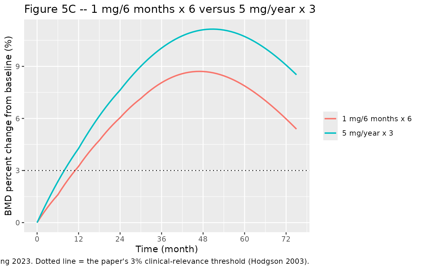
Figure 5A – single dose (a known deviation)
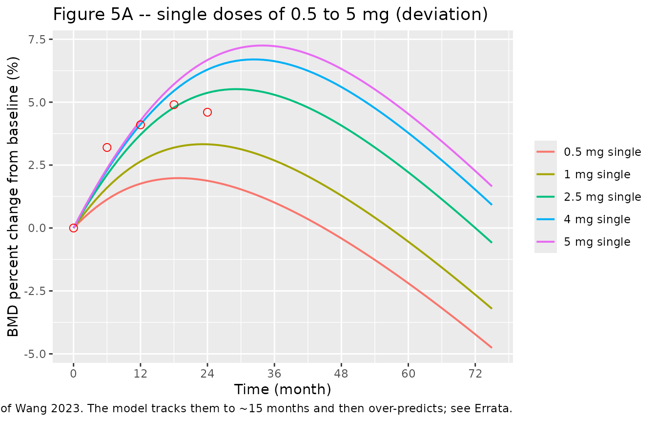
The single-dose panels of Figures 4A and 5A are not reproducible from the printed equations and Table 2 estimates: the packaged model keeps rising to a later, higher peak than the published curves. The plot below shows the disagreement rather than hiding it; the Errata section quantifies it and demonstrates that the paper’s own two panels disagree with each other.
single <- sim_typ |>
  dplyr::filter(grepl("single$", regimen)) |>
  dplyr::mutate(regimen = factor(regimen, levels = REGIMEN_LEVELS))

single |>
  ggplot(aes(time, pct, colour = regimen)) +
  geom_line(linewidth = 0.7) +
  geom_point(data = fig4a_obs, aes(time, pct_obs), inherit.aes = FALSE,
             shape = 21, colour = "red", size = 2.5) +
  scale_x_continuous(breaks = seq(0, 72, by = 12)) +
  labs(
    x = "Time (month)", y = "BMD percent change from baseline (%)",
    colour = NULL,
    title = "Figure 5A -- single doses of 0.5 to 5 mg (deviation)",
    caption = paste(
      "Lines: packaged model, typical value. Red circles: single-dose 5 mg",
      "observations digitised from Figure 4A of Wang 2023. The model tracks",
      "them to ~15 months and then over-predicts; see Errata."
    )
  )
Peak BMD change: model versus the paper’s own simulations
peaks <- sim_typ |>
  dplyr::group_by(regimen) |>
  dplyr::summarise(
    pct_peak_model = max(pct),
    t_peak_model   = time[which.max(pct)],
    pct_72_model   = pct[time == 72],
    .groups = "drop"
  ) |>
  dplyr::left_join(fig5_peaks, by = "regimen") |>
  dplyr::mutate(
    rel_diff_pct = 100 * (pct_peak_model - pct_peak_paper) / pct_peak_paper,
    panel = ifelse(grepl("single$", regimen), "Fig 5A (single dose)", "Fig 5B/5C (multiple dose)")
  ) |>
  dplyr::arrange(panel, match(regimen, REGIMEN_LEVELS))

peaks |>
  dplyr::select(panel, regimen, pct_peak_paper, pct_peak_model, t_peak_model,
                rel_diff_pct, pct_72_model) |>
  dplyr::rename(
    "Panel"                        = panel,
    "Regimen"                      = regimen,
    "Peak, paper figure (%)"       = pct_peak_paper,
    "Peak, packaged model (%)"     = pct_peak_model,
    "Time of model peak (month)"   = t_peak_model,
    "Relative difference (%)"      = rel_diff_pct,
    "Model at 72 months (%)"       = pct_72_model
  ) |>
  knitr::kable(digits = 2,
caption = "Peak BMD percent change: packaged model vs values digitised from Wang 2023 Figure 5.")| Panel | Regimen | Peak, paper figure (%) | Peak, packaged model (%) | Time of model peak (month) | Relative difference (%) | Model at 72 months (%) |
|---|---|---|---|---|---|---|
| Fig 5A (single dose) | 0.5 mg single | 1.95 | 1.98 | 19 | 1.65 | -4.23 |
| Fig 5A (single dose) | 1 mg single | 2.70 | 3.33 | 23 | 23.32 | -2.65 |
| Fig 5A (single dose) | 2.5 mg single | 3.80 | 5.52 | 29 | 45.22 | 0.00 |
| Fig 5A (single dose) | 4 mg single | 4.45 | 6.70 | 32 | 50.50 | 1.52 |
| Fig 5A (single dose) | 5 mg single | 4.65 | 7.25 | 34 | 55.92 | 2.27 |
| Fig 5B/5C (multiple dose) | 0.5 mg/year x 6 | 4.00 | 4.32 | 44 | 8.01 | 3.22 |
| Fig 5B/5C (multiple dose) | 1 mg/year x 6 | 6.90 | 7.32 | 55 | 6.12 | 6.87 |
| Fig 5B/5C (multiple dose) | 2.5 mg/year x 6 | 10.30 | 10.89 | 66 | 5.68 | 10.76 |
| Fig 5B/5C (multiple dose) | 4 mg/year x 6 | 11.90 | 12.19 | 68 | 2.46 | 12.13 |
| Fig 5B/5C (multiple dose) | 5 mg/year x 6 | 12.30 | 12.68 | 68 | 3.12 | 12.64 |
| Fig 5B/5C (multiple dose) | 1 mg/6 months x 6 | 8.35 | 8.71 | 47 | 4.31 | 5.97 |
| Fig 5B/5C (multiple dose) | 5 mg/year x 3 | 10.70 | 11.14 | 51 | 4.16 | 9.07 |
multi <- peaks |> dplyr::filter(panel == "Fig 5B/5C (multiple dose)")

# Deterministic typical-value peaks compared against digitised figure peaks.
# Realised relative differences across the seven multiple-dose regimens are
# +2.5% to +8.0% (largest at the small 0.5 mg peak, where the +/- 0.3 pp
# digitisation error is worth ~8% on its own). The bound is set at 20% so
# digitisation error cannot trip it, while a mis-transcribed rate constant
# (which moves these by 40-100%) still does.
stopifnot(max(abs(multi$rel_diff_pct)) < 20)

# Dose-dependence: deterministic typical-value trajectories, no cohort noise,
# so exact ordering is a legitimate assertion of the paper's central claim
# that "BMD increased in a dose-dependent manner".
annual_peaks <- peaks |>
  dplyr::filter(grepl("/year x 6$", regimen)) |>
  dplyr::arrange(match(regimen, REGIMEN_LEVELS))
stopifnot(all(diff(annual_peaks$pct_peak_model) > 0))
Published claims
pk <- function(r) peaks$pct_peak_model[peaks$regimen == r]
stopifnot(length(pk("5 mg single")) == 1L)   # guard the lookup

claim <- function(text, achieved, pass, deviation = FALSE) {
  tibble::tibble(Claim = text, Achieved = achieved, Pass = pass, Deviation = deviation)
}

claims <- dplyr::bind_rows(
  claim("Single dose: 2.5, 4 and 5 mg each raise BMD by >3% from baseline (Results 3.4)",
        sprintf("peaks %.1f / %.1f / %.1f%%", pk("2.5 mg single"), pk("4 mg single"), pk("5 mg single")),
        all(c(pk("2.5 mg single"), pk("4 mg single"), pk("5 mg single")) > 3)),
  claim("Single dose: 0.5 mg does not reach the 3% threshold (implied by Results 3.4)",
        sprintf("peak %.1f%%", pk("0.5 mg single")),
        pk("0.5 mg single") < 3),
  claim("Single dose: 1 mg does not reach the 3% threshold (implied by Results 3.4)",
        sprintf("peak %.1f%% -- model marginally exceeds 3%%", pk("1 mg single")),
        pk("1 mg single") < 3, deviation = TRUE),
  claim("Twice-yearly 1 mg x 6 achieves a BMD change of 3% (Results 3.4)",
        sprintf("peak %.1f%%", pk("1 mg/6 months x 6")),
        pk("1 mg/6 months x 6") > 3),
  claim("Once-yearly dosing: BMD rises monotonically with dose (Results 3.4)",
        sprintf("peaks %.1f to %.1f%% over 0.5-5 mg", min(annual_peaks$pct_peak_model), max(annual_peaks$pct_peak_model)),
        all(diff(annual_peaks$pct_peak_model) > 0)),
  claim("Recommended regimen (1 mg q6 months x 6) beats once-yearly 1 mg on peak BMD",
        sprintf("%.1f%% vs %.1f%%", pk("1 mg/6 months x 6"), pk("1 mg/year x 6")),
        pk("1 mg/6 months x 6") > pk("1 mg/year x 6")),
  claim("Figure 4A/5A single-dose 5 mg plateau of about 4.65%",
        sprintf("model peak %.1f%% at month %d", pk("5 mg single"),
                as.integer(peaks$t_peak_model[peaks$regimen == "5 mg single"])),
        FALSE, deviation = TRUE)
)

claims |> knitr::kable(caption = "Wang 2023 claims checked against the packaged model.")| Claim | Achieved | Pass | Deviation |
|---|---|---|---|
| Single dose: 2.5, 4 and 5 mg each raise BMD by >3% from baseline (Results 3.4) | peaks 5.5 / 6.7 / 7.3% | TRUE | FALSE |
| Single dose: 0.5 mg does not reach the 3% threshold (implied by Results 3.4) | peak 2.0% | TRUE | FALSE |
| Single dose: 1 mg does not reach the 3% threshold (implied by Results 3.4) | peak 3.3% – model marginally exceeds 3% | FALSE | TRUE |
| Twice-yearly 1 mg x 6 achieves a BMD change of 3% (Results 3.4) | peak 8.7% | TRUE | FALSE |
| Once-yearly dosing: BMD rises monotonically with dose (Results 3.4) | peaks 4.3 to 12.7% over 0.5-5 mg | TRUE | FALSE |
| Recommended regimen (1 mg q6 months x 6) beats once-yearly 1 mg on peak BMD | 8.7% vs 7.3% | TRUE | FALSE |
| Figure 4A/5A single-dose 5 mg plateau of about 4.65% | model peak 7.3% at month 34 | FALSE | TRUE |
Between-study variability
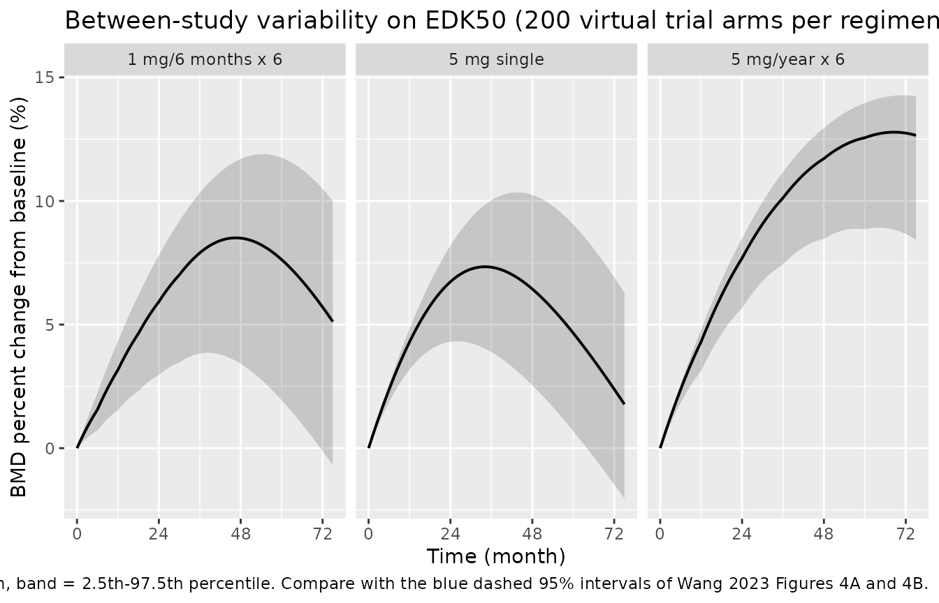
The only random effect is eta_study_lekd50, so simulated
arms differ purely in potency. 200 virtual arms per regimen is the
cohort cap for this library and is ample for an arm-level band.
N_ARMS <- 200L

VPC_REGIMENS <- Filter(
  function(r) r$regimen %in% c("5 mg/year x 6", "1 mg/6 months x 6", "5 mg single"),
  REGIMENS
)
stopifnot(length(VPC_REGIMENS) == 3L)

events_vpc <- dplyr::bind_rows(
  lapply(seq_along(VPC_REGIMENS), function(i) {
    r <- VPC_REGIMENS[[i]]
    make_regimen(r$regimen, r$dose_mg, r$dose_times,
                 n = N_ARMS, id_offset = i * 100000L)
  })
)
stopifnot(!anyDuplicated(unique(events_vpc[, c("id", "time", "evid")])))

sim_vpc <- rxode2::rxSolve(mod, events = events_vpc,
                           keep = c("regimen", "BMD_BL")) |>
  as.data.frame() |>
  dplyr::mutate(pct = 100 * (BMD_LS - BMD_BL) / BMD_BL)

bands <- sim_vpc |>
  dplyr::group_by(regimen, time) |>
  dplyr::summarise(
    lo  = quantile(pct, 0.025, na.rm = TRUE),
    mid = quantile(pct, 0.500, na.rm = TRUE),
    hi  = quantile(pct, 0.975, na.rm = TRUE),
    .groups = "drop"
  )

bands |>
  ggplot(aes(time, mid)) +
  geom_ribbon(aes(ymin = lo, ymax = hi), alpha = 0.2) +
  geom_line(linewidth = 0.7) +
  facet_wrap(~regimen) +
  scale_x_continuous(breaks = seq(0, 72, by = 24)) +
  labs(
    x = "Time (month)", y = "BMD percent change from baseline (%)",
    title = "Between-study variability on EDK50 (200 virtual trial arms per regimen)",
    caption = paste(
      "Line = median arm, band = 2.5th-97.5th percentile. Compare with the",
      "blue dashed 95% intervals of Wang 2023 Figures 4A and 4B."
    )
  )
band_5mg_single <- bands |>
  dplyr::filter(regimen == "5 mg single", time == 24)
band_5mg_single
#> # A tibble: 1 × 5
#>   regimen      time    lo   mid    hi
#>   <chr>       <dbl> <dbl> <dbl> <dbl>
#> 1 5 mg single    24  4.30  6.73  8.20

# Wang 2023 Figure 4A prints its simulated 95% interval at month 24 as roughly
# 3.05% to 7.10% (maintainer-digitised), i.e. a WIDTH of about 4.05 percentage
# points around a median of 4.65%. The width is the quantity that isolates the
# random-effect encoding from the single-dose level deviation documented in the
# Errata, so it is the width that is compared here.
band_width       <- as.numeric(band_5mg_single$hi - band_5mg_single$lo)
band_width_paper <- 7.10 - 3.05
c(model_width_pp = band_width, paper_width_pp = band_width_paper)
#> model_width_pp paper_width_pp
#>       3.891726       4.050000

# Cohort-derived, so this is a loose MAGNITUDE bound, not a tight one.
# It can still go red where it matters: reading omega^2 = 0.4541
# additively rather than exponentially (omega = 0.674 ng/month on an EDK50 of
# 41300 ng/month) collapses the width to ~0, and a factor-of-two error in
# omega^2 moves it outside this range.
stopifnot(band_width > 2, band_width < 8)
Exposure-response analysis of the acute phase reaction
Wang 2023 also reports an exposure-response analysis of the acute phase reaction (APR). It is purely descriptive – observed incidence per dose group, presented as a histogram (Figure 3) and a count table (Table 3) – with no fitted parameters, so there is nothing to encode as a model and the packaged model file covers the K-PD BMD layer only. The published counts are reproduced here for completeness.
# Wang 2023 Table 3, verbatim.
apr <- tibble::tribble(
  ~dose_group, ~study,           ~apr_n, ~total_n,
  "1 mg",      "Grey 2012a",         11,       27,
  "4 mg",      "Shiraki 2017",        6,       12,
  "5 mg",      "Grey 2012b",         27,       20,
  "5 mg",      "Popp 2017",         109,      157,
  "5 mg",      "Sieber 2013",        69,      127,
  "5 mg",      "Li 2022 (a)",       146,      227,
  "5 mg",      "Li 2022 (b)",       158,      231,
  "5 mg",      "Shiraki 2017",        6,       12
)

apr |>
  dplyr::rename("Dose group" = dose_group, "Study" = study,
                "APR (n)" = apr_n, "Total (n)" = total_n) |>
knitr::kable(caption = "Wang 2023 Table 3, incidence of APR by treatment group (verbatim).")| Dose group | Study | APR (n) | Total (n) |
|---|---|---|---|
| 1 mg | Grey 2012a | 11 | 27 |
| 4 mg | Shiraki 2017 | 6 | 12 |
| 5 mg | Grey 2012b | 27 | 20 |
| 5 mg | Popp 2017 | 109 | 157 |
| 5 mg | Sieber 2013 | 69 | 127 |
| 5 mg | Li 2022 (a) | 146 | 227 |
| 5 mg | Li 2022 (b) | 158 | 231 |
| 5 mg | Shiraki 2017 | 6 | 12 |
# Wang 2023 Results 3.3 reports incidences of 40.0%, 50.0% and 65.7% for 1, 4
# and 5 mg. The 1 mg and 4 mg groups reproduce exactly; the 5 mg group cannot,
# because its Grey 2012b row has more events (27) than subjects (20) -- see
# Errata.
reported <- c(`1 mg` = 40.0, `4 mg` = 50.0, `5 mg` = 65.7)
recomputed <- apr |>
  dplyr::group_by(dose_group) |>
  dplyr::summarise(pct = 100 * sum(apr_n) / sum(total_n), .groups = "drop")
recomputed
#> # A tibble: 3 × 2
#>   dose_group   pct
#>   <chr>      <dbl>
#> 1 1 mg        40.7
#> 2 4 mg        50
#> 3 5 mg        66.5

stopifnot(abs(recomputed$pct[recomputed$dose_group == "1 mg"] - reported[["1 mg"]]) < 1)
stopifnot(abs(recomputed$pct[recomputed$dose_group == "4 mg"] - reported[["4 mg"]]) < 1)
stopifnot(any(apr$apr_n > apr$total_n))   # the Table 3 inconsistency is real
Assumptions and deviations
Encoding decisions
-
Dose unit is ng, not mg. Wang 2023 reports
EDK50in ng/month, andIR = KDE * Aonly shares those units if the virtual compartment carries nanograms. A 5 mg infusion is thereforeamt = 5e6. Theunits_checkchunk above states the arithmetic; entering mg instead silences the drug effect entirely (stimulation fraction 1e-5 rather than 0.91). -
EPS = 0.00005is read as a variance, so the additive residual SD issqrt(0.00005) = 0.00707g/cm^2 (about 0.9% of the 0.64-1.06 g/cm^2 baseline range in Table 1). NONMEM$SIGMAis reported as a variance and Methods 2.3 describes the residual as normal with variancesigma^2. Read as an SD instead it would imply 0.006% DXA precision, which no instrument achieves. -
ETA of EDK50is applied exponentially, not additively. Wang 2023 Equation 8 printsKei = TVKe + etai, but that section is generic boilerplate – it is written about “Ke”, “the observed concentration value” and “the individual PK parameters”, none of which exist in this paper’s K-PD BMD model, and the second (residual) equation the sentence promises is missing entirely. Two independent checks favour the exponential reading: (a) additively,omega = sqrt(0.4541) = 0.674ng/month on anEDK50of 41300 ng/month is a coefficient of variation of 0.0016%, which cannot produce the visibly wide simulated 95% bands in Figures 4A and 4B; (b) exponentially it is 75.8% CV, and propagating it throughEDK50gives a 95% band 3.9 percentage points wide at month 24 for a single 5 mg dose, against the 4.0 percentage points digitised from Figure 4A – so the exponential reading reproduces the published spread, which is the part of the figure that depends on the random-effect encoding rather than on the single-dose level deviation described below. -
Tolmultiplies the whole synthesis rate, as printed in Equation 7, including its baseline part rather than only the drug-driven increment. The consequence – an undosed arm drifting below baseline by -6.9% over 72 months, i.e. about -1.16% per year, verified against the closed form in check 2b – is retained because it is the published equation, because the implied untreated bone-loss rate is physiologically plausible, and because it is the mechanism by which the paper’s own low-dose single-administration curves fall back towards and through baseline in Figure 5A. RestrictingTolto the drug-driven increment only (KS * (1 + Tol * f)) would remove that behaviour and is not what Equation 7 prints. -
BASEis encoded as the covariateBMD_BL, not as anini()parameter. Wang 2023 definesBASE = R(0) = KS/KDin Equations 3 and 4 but does not list it in Table 2, because it is supplied per arm from the digitised source trial (Table 1, “Baseline of vertebral BMD”). The model is exactly scale-invariant inBMD_BLfor percent-change output, so no value was invented: this vignette uses 0.81 g/cm^2 (Table 1, Black 2012) purely to fix the absolute axis. -
Zero-variance etas are omitted.
ETA of KDE,ETA of KDandETA of Kare all reported as “FIXED” in Table 2, i.e. held at zero. They are omitted rather than written as~ fixed(0), because a zero-variance diagonal makes OMEGA singular and breaks the Cholesky sampler used byrxSolve. -
Between-study, not between-subject. The analysis
units are published trial arms, so the single random effect is named
eta_study_lekd50per the MBMA convention. The model simulates arm-level mean BMD and must not be read as an individual-level PD model.
Non-paper-derived values
- The reference values in
fig4a_obs,fig4b_obsandfig5_peakswere digitised by the maintainers from Wang 2023 Figures 4 and 5 (page 8 and page 9 of the PDF, rendered at 300-400 dpi and read against the printed axis ticks), with an estimated uncertainty of about +/- 0.3 percentage points. Wang 2023 publishes no numeric table of its simulated trajectories. These values are used only for comparison; no model parameter is derived from them. -
population$race_ethnicityis an inference, not a Wang 2023 field. Wang 2023 reports no race column; the split is the patient-weighted share of the three explicitly East-Asian contributing cohorts (Liang 2017, Li 2022, Nakamura 2017; 963 of 6014 patients) against the remainder.
Errata and deviations from the source
-
The single-dose panels (Figures 4A and 5A) are not
reproducible from Equations 1-7 and Table 2. The packaged model
tracks the digitised single-dose 5 mg observations well to about 15
months (4.3% at month 12 against a digitised 4.1%) and then keeps rising
to a peak of about 7.3% at month 34, whereas the published curve
flattens at about 4.65% by month 18. The mechanism is unambiguous: with
KDE = 0.0815/month the virtual compartment has an 8.5-month half-life, so at month 27 the stimulation fractionIR/(EDK50+IR)is still 0.52, and withKD = 0.00474/month the BMD pool cannot equilibrate against a signal that strong (the equilibrium BMD change implied by a sustained fractionfis100*fpercent). No value ofKDEreproduces both panels. Raising it to 0.35 /month does flatten the single-dose 5 mg curve at about the published level (4.1% peak at month 15), but it then under-predicts the once-yearly peaks of Figure 5B by 8-18% and the 5 mg/year x 3 peak of Figure 5C by 19%; the published 0.0815 /month reproduces all seven multiple-dose peaks to within 8%. - Figures 4A and 4B disagree with each other at month 12. Only one dose has been administered by month 12 in either panel, so the two curves must coincide there. Digitised, Figure 4A reads 4.15% and Figure 4B reads 5.39% – a 30% discrepancy that no parameter set can absorb. The packaged model gives 4.27%, i.e. it agrees with Figure 4A. This is the clearest evidence that the disagreement is in the paper’s figure generation rather than in the reading of its equations, and it is why the multiple-dose panels were chosen as the validation target.
- The paper’s prose about once-yearly low doses contradicts its own Figure 5B. Results 3.4 states that “the change in BMD of 0.5 mg and 1 mg was small”, but Figure 5B shows the 1 mg once-yearly arm peaking near 6.9%, well above the paper’s own 3% relevance threshold. The packaged model gives 7.3%, agreeing with the figure. Following the standing rule that a results figure or table beats a Discussion or prose summary, the figure is treated as the reproduction target.
- Wang 2023 Table 3 row Grey 2012b reports 27 APR events among 20 subjects. More events than subjects is impossible; Grey 2012b randomised 20 patients to 5 mg. The 1 mg and 4 mg group incidences in Results 3.3 (40.0% and 50.0%) recompute exactly from Table 3, but the 5 mg group’s reported 65.7% cannot be recovered from the printed counts (64.7% excluding the impossible row, 66.5% including it). Because the APR analysis is descriptive and contributes no model parameters, this affects nothing in the packaged model; Table 3 is reproduced verbatim above with the inconsistency asserted rather than silently corrected.
-
Model-body prose vs equations. Methods 2.2 says the
synthesis rate “was inhibited by a virtual infusion
rate (IR)”, while Results 3.2 says the same rate is “modeled with a
stimulated Emax model”. Equation 5 prints
(1 + IR/(EDK50+IR)), i.e. stimulation, and stimulation is what raises BMD in every published figure. The equation is encoded. -
No
Emaxparameter. Equation 5 has a fixed unit numerator, so the maximum achievable stimulation of BMD synthesis is exactly two-fold. Table 2 lists noEmax, so none was introduced. -
Toluses absolute time, not time since the last dose. Wang 2023 introduces the term specifically to reproduce attenuation of BMD gain across successive annual doses (Results 3.2, Discussion), which a per-dose reset would not produce; and the absolute-time reading is what reproduces the post-peak decline in Figures 4B, 5B and 5C. - Total hip BMD is not modelled. Trials were included only if they reported both lumbar spine and total hip DXA BMD, but the fitted model, Table 2 and every figure concern lumbar spine BMD alone (“LBMD”). The Discussion explains the choice (higher lumbar-spine bone-turnover rate makes it the preferred surrogate). No total-hip parameters are reported, so none are encoded.
- Supplementary Figures S1-S4 (goodness-of-fit, PRED, IPRED and VPC plots) are diagnostics only and contain no parameter values, so the supplement is not required to reproduce the model.
#> R version 4.6.1 (2026-06-24)
#> Platform: x86_64-pc-linux-gnu
#> Running under: Ubuntu 24.04.5 LTS
#>
#> Matrix products: default
#> BLAS:   /usr/lib/x86_64-linux-gnu/openblas-pthread/libblas.so.3
#> LAPACK: /usr/lib/x86_64-linux-gnu/openblas-pthread/libopenblasp-r0.3.26.so;  LAPACK version 3.12.0
#>
#> locale:
#>  [1] LC_CTYPE=C.UTF-8       LC_NUMERIC=C           LC_TIME=C.UTF-8
#>  [4] LC_COLLATE=C.UTF-8     LC_MONETARY=C.UTF-8    LC_MESSAGES=C.UTF-8
#>  [7] LC_PAPER=C.UTF-8       LC_NAME=C              LC_ADDRESS=C
#> [10] LC_TELEPHONE=C         LC_MEASUREMENT=C.UTF-8 LC_IDENTIFICATION=C
#>
#> time zone: UTC
#> tzcode source: system (glibc)
#>
#> attached base packages:
#> [1] stats     graphics  grDevices utils     datasets  methods   base
#>
#> other attached packages:
#> [1] ggplot2_4.0.3         tidyr_1.3.2           dplyr_1.2.1
#> [4] rxode2_5.1.8          nlmixr2lib_0.3.2.9000
#>
#> loaded via a namespace (and not attached):
#>  [1] gtable_0.3.6        xfun_0.61           bslib_0.12.0
#>  [4] rxode2lincmt_0.1.0  vctrs_0.7.3         tools_4.6.1
#>  [7] generics_0.1.4      parallel_4.6.1      tibble_3.3.1
#> [10] symengine_0.2.14    pkgconfig_2.0.3     data.table_1.18.6.1
#> [13] checkmate_2.3.4     RColorBrewer_1.1-3  S7_0.2.2
#> [16] desc_1.4.3          lifecycle_1.0.5     compiler_4.6.1
#> [19] farver_2.1.2        textshaping_1.0.5   fontawesome_0.5.3
#> [22] htmltools_0.5.9     sys_3.4.3           sass_0.4.10
#> [25] yaml_2.3.12         pillar_1.11.1       pkgdown_2.2.1
#> [28] crayon_1.5.3        jquerylib_0.1.4     whisker_0.4.1
#> [31] openssl_2.4.2       cachem_1.1.0        tidyselect_1.2.1
#> [34] digest_0.6.39       lotri_1.0.5         purrr_1.2.2
#> [37] labeling_0.4.3      rxode2ll_2.0.18     fastmap_1.2.0
#> [40] grid_4.6.1          cli_3.6.6           dparser_1.3.1-14
#> [43] magrittr_2.0.5      utf8_1.2.6          withr_3.0.3
#> [46] scales_1.4.0        backports_1.5.1     rmarkdown_2.32
#> [49] otel_0.2.0          askpass_1.2.1       ragg_1.5.2
#> [52] memoise_2.0.1       evaluate_1.0.5      knitr_1.52
#> [55] rex_1.2.2           PreciseSums_0.7     rlang_1.3.0
#> [58] downlit_0.4.5       Rcpp_1.1.2          glue_1.8.1
#> [61] xml2_1.6.0          jsonlite_2.0.0      R6_2.6.1
#> [64] systemfonts_1.3.2   fs_2.1.0