Ethambutol in adults with tuberculosis and HIV (Ndzamba 2025)
Source:vignettes/articles/Ndzamba_2025_ethambutol.Rmd
Ndzamba_2025_ethambutol.Rmd
library(nlmixr2lib)
library(rxode2)
library(PKNCA)
library(dplyr)
library(ggplot2)

rxode2::rxSetSeed(20250211)
set.seed(20250211)
Ndzamba et al. (2025) modelled ethambutol pharmacokinetics in 61 South African adults with newly diagnosed drug-susceptible pulmonary tuberculosis and HIV from the TB-HAART study, and used the model to evaluate the WHO weight-band doses for the 275 mg first-line fixed-dose combination and the 400 mg tablet used in MDR-TB regimens.
mod <- nlmixr2lib::readModelDb("Ndzamba_2025_ethambutol")Reference: Ndzamba B, Denti P, McIlleron H, Smith P, Mthiyane T, Rustomjee R, Onyebujoh P, Resendiz-Galvan JE, Wasserman S (2025). Pharmacokinetics of ethambutol and weight banded dosing in South African adults newly diagnosed with tuberculosis and HIV. Antimicrob Agents Chemother 69(2):e01200-24. doi:10.1128/aac.01200-24
Population
| Characteristic | Overall (N = 61) |
|---|---|
| Age (years) | 32.0 [27-37] |
| Female | 33 (54.1%) |
| Weight (kg) | 55.2 [50.0-62.4] |
| Height (m) | 1.59 [1.54-1.68] |
| Fat-free mass (kg) | 42 [36.3-45.5] |
| CD4+ T-cell count (cells/uL) | 254 [159-323] |
| Creatinine clearance (mL/min) | 97 [80.1-117] |
| e-275 Rifafour formulation | 54 (88.5%) |
| Started ART on day 13 | 41 (67.2%) |
Values are median [IQR] or n (%), reproducing Table 1 of the source. All participants were HIV-positive and ART-naive at enrolment. Ethambutol was given once daily after an overnight fast in a four-drug fixed-dose combination with 275 mg ethambutol hydrochloride per tablet, by weight band: 550 mg below 37.9 kg (1 participant), 825 mg for 38-54.9 kg (31), 1100 mg for 55-70 kg (19) and 1375 mg above 70 kg (10). PK visits were on days 0, 7, 14 and 28, with samples at 1, 1.5, 2, 4, 8 and 12 h after the observed dose and pre-dose samples on days 7, 14 and 28 (plus one on day 13).
Doses in the model are mg of ethambutol base: the
authors converted the hydrochloride dose with the salt factor 0.737 (MW
204.31 / 277.23), so each 275 mg tablet is 202.68 mg of base. Convert a
hydrochloride dose the same way before simulation. Doses go into
transit1, the first of the four transit compartments, not
into depot.
Source trace
Every ini() value carries an in-file comment naming its
source location; this table is the vignette-level summary.
| Quantity | Value | Source |
|---|---|---|
| Structure | 2-compartment; 4 transit compartments (NN = 3) into an absorption compartment | Results; Figure S2; supplementary control stream $MODEL
(ADVAN5, 7 compartments) |
| CL/F, Vc/F (FFM 42 kg) | 34.8 L/h, 156 L | Table 2 + footnote c; control stream TVFFM = 42
|
| Q/F, Vp/F (WT 57 kg) | 34.4 L/h, 564 L | Table 2 + footnote d; control stream TVWT = 57
|
| ka, MTT, NN | 0.877 1/h, 0.717 h, 3 fixed | Table 2; control stream KTR = (NN+1)/MTT
|
| F | 1 fixed | Table 2 |
| Allometry | FFM on CL and Vc, total weight on Q and Vp; exponents 0.75 / 1 fixed | Methods; Results; control stream ALLMCL_FFM,
ALLMV_FFM, ALLMCL_WT,
ALLMV_WT
|
| FFM equation | Janmahasatian, sex-specific constants, height in m | Control stream $PK
|
| Antib-4 effect | F x 1.260, MTT x 1.371 | Table 2; control stream THETA(14),
THETA(15)
|
| BSV CL | 19.9% | Table 2 |
| BOV ka / F / MTT | 52.8% / 27.8% / 66.3% | Table 2 values assigned by the control stream $PK (see
Assumptions) |
| BOV inflation for unobserved doses | 2.20-fold | Table 2 + footnote b; control stream ExtraBOV
|
| Residual error | 24.8% proportional + 0.02 mg/L additive (fixed) | Table 2 + footnote f |
The supplementary control stream fixes the structure, the covariate
equations and the random-effect layout. Its $THETA /
$OMEGA values are initial estimates carried from an earlier
run (for example the Antib-4 effect on MTT starts at 0.01), so Table 2
supplies every value.
Structural verification
These are identities of the published parameterisation, comparing the model’s own typical-value solve with itself, so they are asserted tightly.
# Daily ethambutol doses (mg base) into transit1, observations on the central
# compartment over the last 24 h interval (rxode2 returns Cc at those rows).
ss_events <- function(subj, n_days = 14, obs_step = 0.25) {
  last <- 24 * (n_days - 1)
  doses <- subj |>
    dplyr::select(id, amt) |>
    dplyr::cross_join(data.frame(time = seq(0, last, by = 24))) |>
    dplyr::mutate(evid = 1L, cmt = "transit1")
  obs <- subj |>
    dplyr::select(id) |>
    dplyr::cross_join(data.frame(time = seq(last, last + 24, by = obs_step))) |>
    dplyr::mutate(amt = NA_real_, evid = 0L, cmt = "central")
  dplyr::bind_rows(doses, obs) |>
    dplyr::arrange(id, time, dplyr::desc(evid)) |>
    dplyr::left_join(dplyr::select(subj, -amt), by = "id")
}

trap <- function(time, conc) {
  sum(diff(time) * (utils::head(conc, -1) + utils::tail(conc, -1)) / 2)
}

typical <- function(cov, amt = 1100 * 0.737) {
  ev <- ss_events(data.frame(id = 1L, amt = amt, cov), obs_step = 0.02)
  out <- rxode2::rxSolve(
    rxode2::zeroRe(mod), ev,
    returnType = "data.frame", rtol = 1e-10, atol = 1e-12
  )
  out[out$time >= 312 & !duplicated(out$time), ]
}

ref_adult <- data.frame(
  WT = 49, HT = 160, SEXF = 0, FORM_EMB_ANTIB4 = 0, OCC = 1, SELFADMIN = 0
)
Steady-state mass balance and the reference
individual. Over one steady-state interval the eliminated
amount equals the absorbed dose, so CL * AUCtau = F * Dose.
This pins the unit chain (mg, L, mg/L) and confirms that the transit
chain delivers the whole dose. A 49 kg, 160 cm man has a Janmahasatian
fat-free mass of 42.0 kg, the reference FFM, so his clearance is the
Table 2 value of 34.8 L/h. (A 57 kg, 162 cm woman, at the reference
total weight, has an FFM of only 37.5 kg.)
tv <- typical(ref_adult)
#> ℹ parameter labels from comments will be replaced by 'label()'
#> Warning: some etas defaulted to non-mu referenced, possible parsing error: etaiov_ka_1, etaiov_ka_2, etaiov_ka_3, etaiov_ka_4, etaiov_ka_5, etaiov_ka_6, etaiov_ka_7, etaiov_fdepot_1, etaiov_fdepot_2, etaiov_fdepot_3, etaiov_fdepot_4, etaiov_fdepot_5, etaiov_fdepot_6, etaiov_fdepot_7, etaiov_mtt_1, etaiov_mtt_2, etaiov_mtt_3, etaiov_mtt_4, etaiov_mtt_5, etaiov_mtt_6, etaiov_mtt_7
#> as a work-around try putting the mu-referenced expression on a simple line
#> Warning: some etas defaulted to non-mu referenced, possible parsing error: etaiov_ka_1, etaiov_ka_2, etaiov_ka_3, etaiov_ka_4, etaiov_ka_5, etaiov_ka_6, etaiov_ka_7, etaiov_fdepot_1, etaiov_fdepot_2, etaiov_fdepot_3, etaiov_fdepot_4, etaiov_fdepot_5, etaiov_fdepot_6, etaiov_fdepot_7, etaiov_mtt_1, etaiov_mtt_2, etaiov_mtt_3, etaiov_mtt_4, etaiov_mtt_5, etaiov_mtt_6, etaiov_mtt_7
#> as a work-around try putting the mu-referenced expression on a simple line
#> ℹ omega/sigma items treated as zero: 'etalcl', 'etaiov_ka_1', 'etaiov_ka_2', 'etaiov_ka_3', 'etaiov_ka_4', 'etaiov_ka_5', 'etaiov_ka_6', 'etaiov_ka_7', 'etaiov_fdepot_1', 'etaiov_fdepot_2', 'etaiov_fdepot_3', 'etaiov_fdepot_4', 'etaiov_fdepot_5', 'etaiov_fdepot_6', 'etaiov_fdepot_7', 'etaiov_mtt_1', 'etaiov_mtt_2', 'etaiov_mtt_3', 'etaiov_mtt_4', 'etaiov_mtt_5', 'etaiov_mtt_6', 'etaiov_mtt_7'
mass <- tv$cl[1] * trap(tv$time, tv$Cc) / (tv$fdepot[1] * 1100 * 0.737)
stopifnot(
  abs(mass - 1) < 1e-3,
  abs(tv$ffm[1] - 42) < 0.05,
  abs(tv$cl[1] / 34.8 - 1) < 0.002,
  identical(
    rxode2::rxode2(mod)$state,
    c("transit1", "transit2", "transit3", "transit4", "depot", "central",
      "peripheral1")
  )
)
#> ℹ parameter labels from comments will be replaced by 'label()'
#> Warning: some etas defaulted to non-mu referenced, possible parsing error: etaiov_ka_1, etaiov_ka_2, etaiov_ka_3, etaiov_ka_4, etaiov_ka_5, etaiov_ka_6, etaiov_ka_7, etaiov_fdepot_1, etaiov_fdepot_2, etaiov_fdepot_3, etaiov_fdepot_4, etaiov_fdepot_5, etaiov_fdepot_6, etaiov_fdepot_7, etaiov_mtt_1, etaiov_mtt_2, etaiov_mtt_3, etaiov_mtt_4, etaiov_mtt_5, etaiov_mtt_6, etaiov_mtt_7
#> as a work-around try putting the mu-referenced expression on a simple line
c(ffm_kg = tv$ffm[1], cl_L_h = tv$cl[1], cl_auc_over_f_dose = mass)
#>             ffm_kg             cl_L_h cl_auc_over_f_dose
#>         42.0022718         34.8014117          0.9999842
Formulation identities. Antib-4 raises bioavailability by 26.0%, so the steady-state AUC rises by exactly that factor, and lengthens the mean transit time by 37.1%, which delays the peak.
tv_antib4 <- typical(transform(ref_adult, FORM_EMB_ANTIB4 = 1))
#> ℹ parameter labels from comments will be replaced by 'label()'
#> Warning: some etas defaulted to non-mu referenced, possible parsing error: etaiov_ka_1, etaiov_ka_2, etaiov_ka_3, etaiov_ka_4, etaiov_ka_5, etaiov_ka_6, etaiov_ka_7, etaiov_fdepot_1, etaiov_fdepot_2, etaiov_fdepot_3, etaiov_fdepot_4, etaiov_fdepot_5, etaiov_fdepot_6, etaiov_fdepot_7, etaiov_mtt_1, etaiov_mtt_2, etaiov_mtt_3, etaiov_mtt_4, etaiov_mtt_5, etaiov_mtt_6, etaiov_mtt_7
#> as a work-around try putting the mu-referenced expression on a simple line
#> Warning: some etas defaulted to non-mu referenced, possible parsing error: etaiov_ka_1, etaiov_ka_2, etaiov_ka_3, etaiov_ka_4, etaiov_ka_5, etaiov_ka_6, etaiov_ka_7, etaiov_fdepot_1, etaiov_fdepot_2, etaiov_fdepot_3, etaiov_fdepot_4, etaiov_fdepot_5, etaiov_fdepot_6, etaiov_fdepot_7, etaiov_mtt_1, etaiov_mtt_2, etaiov_mtt_3, etaiov_mtt_4, etaiov_mtt_5, etaiov_mtt_6, etaiov_mtt_7
#> as a work-around try putting the mu-referenced expression on a simple line
#> ℹ omega/sigma items treated as zero: 'etalcl', 'etaiov_ka_1', 'etaiov_ka_2', 'etaiov_ka_3', 'etaiov_ka_4', 'etaiov_ka_5', 'etaiov_ka_6', 'etaiov_ka_7', 'etaiov_fdepot_1', 'etaiov_fdepot_2', 'etaiov_fdepot_3', 'etaiov_fdepot_4', 'etaiov_fdepot_5', 'etaiov_fdepot_6', 'etaiov_fdepot_7', 'etaiov_mtt_1', 'etaiov_mtt_2', 'etaiov_mtt_3', 'etaiov_mtt_4', 'etaiov_mtt_5', 'etaiov_mtt_6', 'etaiov_mtt_7'
auc_ratio <- trap(tv_antib4$time, tv_antib4$Cc) / trap(tv$time, tv$Cc)
tmax_ref <- tv$time[which.max(tv$Cc)] - 312
tmax_antib4 <- tv_antib4$time[which.max(tv_antib4$Cc)] - 312
stopifnot(
  abs(auc_ratio - 1.26) < 1e-3,
  abs(tv_antib4$mtt[1] / tv$mtt[1] - 1.371) < 1e-6,
  tmax_antib4 > tmax_ref
)
c(
  AUC_ratio_Antib4 = auc_ratio, Tmax_Rifafour_h = tmax_ref,
  Tmax_Antib4_h = tmax_antib4
)
#> AUC_ratio_Antib4  Tmax_Rifafour_h    Tmax_Antib4_h
#>             1.26             2.44             2.78
Visual predictive check of the study visits (Figure 1)
A virtual TB-HAART cohort of 200 participants: 54.1% women, weight
log-normal around the Table 1 median of 55.2 kg (IQR 50.0-62.4), heights
normal by sex, 11.5% on Antib-4, and the study’s weight-band doses. The
day-0 dose is occasion 1 and observed. For day 7, the six daily home
doses before the visit are an unobserved occasion (OCC = 2,
SELFADMIN = 1), which produces the pre-dose sample, and the
clinic dose on day 7 is occasion 3 (observed). Percentiles include
residual error (sim).
salt_dose <- function(wt) {
  dplyr::case_when(wt < 38 ~ 550, wt < 55 ~ 825, wt <= 70 ~ 1100, TRUE ~ 1375)
}

# Heights (cm) are normal by sex with a 6.5 cm SD; ht_f / ht_m are the means.
draw_adults <- function(n, wt_median, wt_sdlog, p_female, ht_f, ht_m) {
  sexf <- stats::rbinom(n, 1, p_female)
  data.frame(
    WT = stats::rlnorm(n, log(wt_median), wt_sdlog),
    SEXF = sexf,
    HT = ifelse(sexf == 1, stats::rnorm(n, ht_f, 6.5), stats::rnorm(n, ht_m, 6.5))
  )
}
n_vpc <- 200
vpc_cohort <- draw_adults(n_vpc, 55.2, log(62.4 / 50.0) / 1.349, 0.541, 155, 165) |>
  dplyr::mutate(
    id = dplyr::row_number(),
    FORM_EMB_ANTIB4 = stats::rbinom(n_vpc, 1, 0.115),
    amt = salt_dose(WT) * 0.737
  )

day0 <- vpc_cohort |>
  dplyr::select(id, amt) |>
  dplyr::mutate(time = 0, evid = 1L, cmt = "transit1", OCC = 1, SELFADMIN = 0) |>
  dplyr::bind_rows(
    vpc_cohort |>
      dplyr::select(id) |>
      dplyr::cross_join(data.frame(time = seq(0, 12, by = 0.25))) |>
      dplyr::mutate(amt = NA_real_, evid = 0L, cmt = "central", OCC = 1,
                    SELFADMIN = 0)
  )
day7 <- vpc_cohort |>
  dplyr::select(id, amt) |>
  dplyr::cross_join(data.frame(time = seq(24, 168, by = 24))) |>
  dplyr::mutate(
    evid = 1L, cmt = "transit1",
    OCC = ifelse(time < 168, 2, 3), SELFADMIN = ifelse(time < 168, 1, 0)
  ) |>
  dplyr::bind_rows(
    vpc_cohort |>
      dplyr::select(id) |>
      dplyr::cross_join(data.frame(time = c(167.9, seq(168, 180, by = 0.25)))) |>
      dplyr::mutate(
        amt = NA_real_, evid = 0L, cmt = "central",
        OCC = ifelse(time < 168, 2, 3), SELFADMIN = ifelse(time < 168, 1, 0)
      )
  )
vpc_ev <- dplyr::bind_rows(day0, day7) |>
  dplyr::arrange(id, time, dplyr::desc(evid)) |>
  dplyr::left_join(
    dplyr::select(vpc_cohort, id, WT, HT, SEXF, FORM_EMB_ANTIB4),
    by = "id"
  )

vpc_sim <- rxode2::rxSolve(mod, vpc_ev, returnType = "data.frame")
#> ℹ parameter labels from comments will be replaced by 'label()'
#> Warning: some etas defaulted to non-mu referenced, possible parsing error: etaiov_ka_1, etaiov_ka_2, etaiov_ka_3, etaiov_ka_4, etaiov_ka_5, etaiov_ka_6, etaiov_ka_7, etaiov_fdepot_1, etaiov_fdepot_2, etaiov_fdepot_3, etaiov_fdepot_4, etaiov_fdepot_5, etaiov_fdepot_6, etaiov_fdepot_7, etaiov_mtt_1, etaiov_mtt_2, etaiov_mtt_3, etaiov_mtt_4, etaiov_mtt_5, etaiov_mtt_6, etaiov_mtt_7
#> as a work-around try putting the mu-referenced expression on a simple line
stopifnot(!anyNA(vpc_sim$Cc))

vpc <- vpc_sim |>
  dplyr::mutate(
    visit = ifelse(time <= 12, "Day 0", "Day 7"),
    tad = ifelse(time <= 12, time, time - 168)
  ) |>
  dplyr::group_by(visit, tad) |>
  dplyr::summarise(
    p05 = quantile(sim, 0.05), p50 = median(sim), p95 = quantile(sim, 0.95),
    med_ipred = median(Cc),
    .groups = "drop"
  )
vpc |>
  dplyr::filter(!(visit == "Day 0" & tad < 0.5)) |>
  ggplot(aes(tad, p50)) +
  geom_ribbon(aes(ymin = p05, ymax = p95), alpha = 0.2, fill = "steelblue") +
  geom_line(colour = "steelblue4") +
  facet_wrap(~visit) +
  scale_y_log10() +
  labs(x = "Time after dose (h)", y = "Ethambutol (mg/L)") +
  theme_bw()
#> Warning in transformation$transform(x): NaNs produced
#> Warning in scale_y_log10(): log-10 transformation introduced infinite values.
#> Warning: Removed 1 row containing missing values or values outside the scale range
#> (`geom_ribbon()`).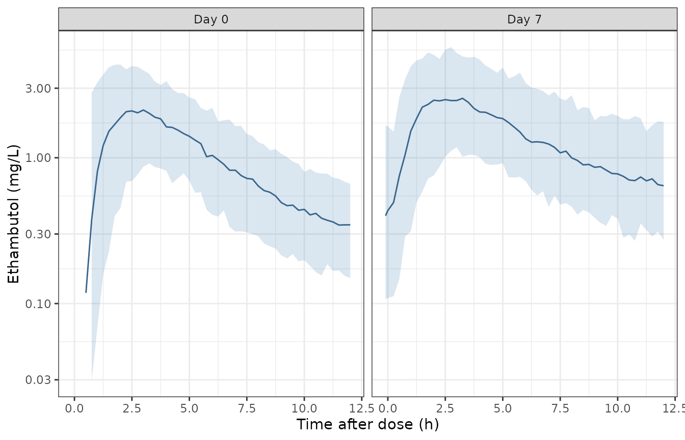
Simulated ethambutol concentrations on day 0 and day 7 (median and 5th-95th percentiles, with residual error); the pre-dose point of day 7 follows the unobserved home dose. Compare with Figure 1 of Ndzamba 2025.
Figure 1 of the paper shows observed medians that peak near 2 mg/L between 2 and 4 h on both visits and fall to about 0.3 mg/L at 12 h on day 0, with day-7 pre-dose medians near 0.3 mg/L.
vpc_at <- function(v, t) {
  x <- vpc$med_ipred[vpc$visit == v & abs(vpc$tad - t) < 1e-6]
  if (length(x) != 1L) stop("no unique VPC row for ", v, " at ", t, " h")
  x
}
vpc_points <- c(
  day0_2h = vpc_at("Day 0", 2), day0_12h = vpc_at("Day 0", 12),
  day7_predose = vpc_at("Day 7", -0.1), day7_2h = vpc_at("Day 7", 2)
)
stopifnot(
  # Centre of the simulated distribution against the observed medians of
  # Figure 1, read by eye (about 2, 0.3, 0.3 and 2 mg/L). A mis-scaled
  # clearance, volume or dose conversion moves these by tens of percent.
  vpc_points[["day0_2h"]] > 1.3, vpc_points[["day0_2h"]] < 3,
  vpc_points[["day0_12h"]] > 0.2, vpc_points[["day0_12h"]] < 0.5,
  vpc_points[["day7_predose"]] > 0.15, vpc_points[["day7_predose"]] < 0.6,
  vpc_points[["day7_2h"]] > 1.3, vpc_points[["day7_2h"]] < 3.5
)
vpc_points
#>      day0_2h     day0_12h day7_predose      day7_2h
#>    1.9663277    0.3414930    0.4187906    2.6210975
Weight-band dosing (Figure 2, Figure S5 and Table 4)
The paper simulated steady-state exposure in 1,225 virtual adults
with TB (Table S2: 56.3% male, weight 52.4 [46.2-58.7] kg, height 1.64
[1.58-1.70] m, FFM 38.1 [34.3-42.4] kg) and compared AUC0-24 with 16-29
mg*h/L and Cmax with 2-6 mg/L. Here a pool is drawn to match Table S2
and 150 adults per weight band are sampled from it, so the lightest band
is filled as well. Every dose is observed (SELFADMIN = 0)
and the formulation is e-275 Rifafour.
pool <- draw_adults(20000, 52.4, log(58.7 / 46.2) / 1.349, 0.437, 159, 168)
pool_ffm <- with(
  pool,
  ifelse(SEXF == 1, 37.99, 42.92) * (HT / 100)^2 * WT /
    (ifelse(SEXF == 1, 35.98, 30.93) * (HT / 100)^2 + WT)
)
data.frame(
  quantity = c("Weight (kg)", "Height (m)", "FFM (kg)"),
  simulated = c(
    sprintf("%.1f [%.1f-%.1f]", median(pool$WT), quantile(pool$WT, 0.25), quantile(pool$WT, 0.75)),
    sprintf("%.2f [%.2f-%.2f]", median(pool$HT / 100), quantile(pool$HT / 100, 0.25), quantile(pool$HT / 100, 0.75)),
    sprintf("%.1f [%.1f-%.1f]", median(pool_ffm), quantile(pool_ffm, 0.25), quantile(pool_ffm, 0.75))
  ),
  table_s2 = c("52.4 [46.2-58.7]", "1.64 [1.58-1.70]", "38.1 [34.3-42.4]")
) |>
  dplyr::rename("Characteristic" = quantity, "Simulated pool" = simulated,
                "Table S2" = table_s2) |>
knitr::kable(caption = "Virtual simulation population, median [IQR].")| Characteristic | Simulated pool | Table S2 |
|---|---|---|
| Weight (kg) | 52.4 [46.6-59.2] | 52.4 [46.2-58.7] |
| Height (m) | 1.64 [1.59-1.70] | 1.64 [1.58-1.70] |
| FFM (kg) | 40.7 [35.5-46.2] | 38.1 [34.3-42.4] |
Weight and height match Table S2, but the pool’s fat-free mass is a few kg above the tabulated 38.1 kg. Table S2’s FFM cannot be reproduced from its own weight, height and sex medians: a 52.4 kg, 1.64 m man already has a Janmahasatian FFM of 44.6 kg and a woman of the same size 35.9 kg, so the source population must pair lower weights with men than an independent draw does. The pool is left matched to the tabulated weight, height and sex, and is not tuned to the FFM.
arms <- data.frame(
  tablet = c(rep("275 mg (DS-TB)", 6), rep("400 mg (MDR-TB)", 4)),
  band = c("<37.9", "<37.9", "38-54.9", "38-54.9", "55-70", ">70",
           "30-45.9", "30-45.9", "46-70", ">70"),
  lo = c(25, 25, 38, 38, 55, 70, 30, 30, 46, 70),
  hi = c(38, 38, 55, 55, 70, 120, 46, 46, 70, 120),
  regimen = c("WHO", "Proposed", "WHO", "Proposed", "WHO", "WHO",
              "WHO", "Proposed", "WHO", "WHO"),
  salt_mg = c(550, 825, 825, 1100, 1100, 1375, 800, 1200, 1200, 1600)
) |>
  dplyr::mutate(arm = paste(tablet, band, regimen, salt_mg))

n_band <- 150
band_cohort <- arms |>
  dplyr::rowwise() |>
  dplyr::reframe(
    arm = arm,
    row = sample(which(pool$WT >= lo & pool$WT < hi), n_band, replace = TRUE)
  ) |>
  dplyr::mutate(WT = pool$WT[row], HT = pool$HT[row], SEXF = pool$SEXF[row]) |>
  dplyr::left_join(arms, by = "arm") |>
  dplyr::mutate(
    id = dplyr::row_number(), amt = salt_mg * 0.737,
    FORM_EMB_ANTIB4 = 0, OCC = 1, SELFADMIN = 0
  )

band_ev <- ss_events(
  dplyr::select(band_cohort, id, amt, WT, HT, SEXF, FORM_EMB_ANTIB4, OCC,
                SELFADMIN)
)
band_sim <- rxode2::rxSolve(mod, band_ev, returnType = "data.frame") |>
  dplyr::filter(time >= 312)
stopifnot(!anyNA(band_sim$Cc))
PKNCA validation
conc <- band_sim |>
  dplyr::filter(!is.na(Cc)) |>
  dplyr::mutate(tad = time - 312) |>
  dplyr::left_join(dplyr::select(band_cohort, id, arm), by = "id") |>
  dplyr::select(id, arm, tad, Cc)
dose <- band_cohort |>
  dplyr::transmute(id, arm, tad = 0, amt)

conc_obj <- PKNCA::PKNCAconc(conc, Cc ~ tad | arm + id)
dose_obj <- PKNCA::PKNCAdose(dose, amt ~ tad | arm + id)
intervals <- data.frame(start = 0, end = 24, cmax = TRUE, auclast = TRUE)
nca <- PKNCA::pk.nca(PKNCA::PKNCAdata(conc_obj, dose_obj, intervals = intervals))
nca_res <- as.data.frame(nca$result)

band_exp <- nca_res |>
  dplyr::filter(PPTESTCD %in% c("cmax", "auclast")) |>
  dplyr::select(id, arm, PPTESTCD, PPORRES) |>
  tidyr::pivot_wider(names_from = PPTESTCD, values_from = PPORRES) |>
  dplyr::left_join(arms, by = "arm")
The published medians below were read by the maintainers from the box plots of Figure 2 (275 mg tablet) and Figure S5 (400 mg tablet); the paper does not tabulate them. The Cmax panel of Figure S5 labels its heavier bands 46-55 and >55 kg, unlike its AUC panel (46-70 and >70 kg); the AUC-panel bands are used.
published <- data.frame(
  arm = arms$arm,
  auclast = c(14.3, 21.4, 18.4, 24.6, 22.0, 24.1, 19.5, 29.2, 25.6, 28.1),
  cmax = c(1.82, 2.57, 2.21, 2.90, 2.54, 2.65, 2.35, 3.45, 3.00, 3.06)
)
stopifnot(all(published$arm %in% band_exp$arm))
cmp <- nlmixr2lib::ncaComparisonTable(
  simulated = dplyr::filter(nca_res, PPTESTCD %in% c("cmax", "auclast")),
  reference = published,
  by = "arm",
  units = c(cmax = "mg/L", auclast = "mg*h/L"),
  tolerance_pct = 20
)
cmp |>
  dplyr::rename("Arm (tablet, band, regimen, mg salt)" = arm) |>
knitr::kable(caption = "Simulated vs Figure 2 / Figure S5 median steady-state AUC0-24 and Cmax.")| NCA parameter | Arm (tablet, band, regimen, mg salt) | Reference | Simulated | % diff |
|---|---|---|---|---|
| Cmax (mg/L) | 275 mg (DS-TB) <37.9 WHO 550 | 1.82 | 1.84 | +1.1% |
| Cmax (mg/L) | 275 mg (DS-TB) <37.9 Proposed 825 | 2.57 | 2.76 | +7.3% |
| Cmax (mg/L) | 275 mg (DS-TB) 38-54.9 WHO 825 | 2.21 | 2.4 | +8.5% |
| Cmax (mg/L) | 275 mg (DS-TB) 38-54.9 Proposed 1100 | 2.9 | 3.13 | +7.9% |
| Cmax (mg/L) | 275 mg (DS-TB) 55-70 WHO 1100 | 2.54 | 2.81 | +10.5% |
| Cmax (mg/L) | 275 mg (DS-TB) >70 WHO 1375 | 2.65 | 2.99 | +12.9% |
| Cmax (mg/L) | 400 mg (MDR-TB) 30-45.9 WHO 800 | 2.35 | 2.46 | +4.8% |
| Cmax (mg/L) | 400 mg (MDR-TB) 30-45.9 Proposed 1200 | 3.45 | 3.64 | +5.4% |
| Cmax (mg/L) | 400 mg (MDR-TB) 46-70 WHO 1200 | 3 | 3.02 | +0.5% |
| Cmax (mg/L) | 400 mg (MDR-TB) >70 WHO 1600 | 3.06 | 3.5 | +14.4% |
| AUClast (mg*h/L) | 275 mg (DS-TB) <37.9 WHO 550 | 14.3 | 14.2 | -0.8% |
| AUClast (mg*h/L) | 275 mg (DS-TB) <37.9 Proposed 825 | 21.4 | 21.7 | +1.2% |
| AUClast (mg*h/L) | 275 mg (DS-TB) 38-54.9 WHO 825 | 18.4 | 17.8 | -3.3% |
| AUClast (mg*h/L) | 275 mg (DS-TB) 38-54.9 Proposed 1100 | 24.6 | 25.4 | +3.1% |
| AUClast (mg*h/L) | 275 mg (DS-TB) 55-70 WHO 1100 | 22 | 22.7 | +3.3% |
| AUClast (mg*h/L) | 275 mg (DS-TB) >70 WHO 1375 | 24.1 | 25.8 | +7.0% |
| AUClast (mg*h/L) | 400 mg (MDR-TB) 30-45.9 WHO 800 | 19.5 | 19.4 | -0.4% |
| AUClast (mg*h/L) | 400 mg (MDR-TB) 30-45.9 Proposed 1200 | 29.2 | 29 | -0.8% |
| AUClast (mg*h/L) | 400 mg (MDR-TB) 46-70 WHO 1200 | 25.6 | 25.3 | -1.3% |
| AUClast (mg*h/L) | 400 mg (MDR-TB) >70 WHO 1600 | 28.1 | 29.3 | +4.4% |
band_long <- band_exp |>
  tidyr::pivot_longer(c(auclast, cmax), names_to = "metric") |>
  dplyr::mutate(
    metric = factor(metric, levels = c("auclast", "cmax"),
                    labels = c("AUC0-24 (mg*h/L)", "Cmax (mg/L)")),
    band = factor(
      band,
      levels = c("<37.9", "38-54.9", "30-45.9", "46-70", "55-70", ">70")
    ),
    regimen = factor(regimen, levels = c("WHO", "Proposed"))
  )
ref_ranges <- data.frame(
  metric = factor(c("AUC0-24 (mg*h/L)", "Cmax (mg/L)"),
                  levels = levels(band_long$metric)),
  lo = c(16, 2), hi = c(29, 6)
)
ggplot(band_long, aes(band, value, fill = regimen)) +
  geom_rect(data = ref_ranges, aes(xmin = -Inf, xmax = Inf, ymin = lo, ymax = hi),
            inherit.aes = FALSE, alpha = 0.2, fill = "grey50") +
  geom_boxplot(outlier.size = 0.4) +
  facet_grid(metric ~ tablet, scales = "free") +
  labs(x = "Weight band (kg)", y = NULL, fill = NULL) +
  theme_bw()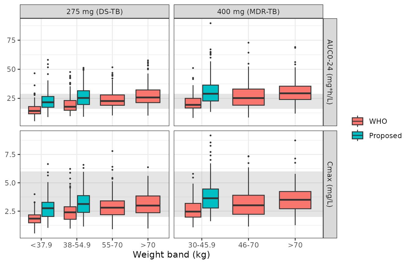
Simulated steady-state ethambutol AUC0-24 (top) and Cmax (bottom) by weight band for the WHO and proposed doses; shaded bands are the 16-29 mg*h/L and 2-6 mg/L reference ranges. Replicates Figure 2 (275 mg tablet) and Figure S5 (400 mg tablet) of Ndzamba 2025.
Median AUC0-24 agrees with the figures to within a few percent in every arm. Median Cmax runs up to about 15% above them, most in the heavier bands, while AUC0-24 does not. The paper does not state the time grid from which its simulated Cmax was read; a coarser grid than the 15-minute grid used here would read a lower peak.
The paper’s conclusions (Results, Table 4): with WHO doses, the bands below 55 kg (275 mg tablet) and below 46 kg (400 mg tablet) have lower exposure than the heavier bands, and one extra tablet brings the 275 mg-tablet bands’ median AUC0-24 into the 16-29 mgh/L range. For the 400 mg tablet, the proposed 1200 mg dose puts the lightest band’s median at the upper edge of that range, about 29 mgh/L, both in Figure S5 and here, so only its lower bound is checked.
band_med <- band_exp |>
  dplyr::group_by(arm, tablet, band, regimen) |>
  dplyr::summarise(
    auc = median(auclast), cmax = median(cmax),
    sdlog_auc = sd(log(auclast)), .groups = "drop"
  )
band_med |>
  dplyr::select(-arm) |>
  dplyr::rename("Tablet" = tablet, "Band (kg)" = band, "Regimen" = regimen,
                "Median AUC0-24" = auc, "Median Cmax" = cmax,
                "SD of log AUC0-24" = sdlog_auc) |>
knitr::kable(digits = 2, caption = "Simulated steady-state exposure by arm.")| Tablet | Band (kg) | Regimen | Median AUC0-24 | Median Cmax | SD of log AUC0-24 |
|---|---|---|---|---|---|
| 275 mg (DS-TB) | 38-54.9 | Proposed | 25.35 | 3.13 | 0.34 |
| 275 mg (DS-TB) | 38-54.9 | WHO | 17.80 | 2.40 | 0.34 |
| 275 mg (DS-TB) | 55-70 | WHO | 22.72 | 2.81 | 0.32 |
| 275 mg (DS-TB) | <37.9 | Proposed | 21.65 | 2.76 | 0.37 |
| 275 mg (DS-TB) | <37.9 | WHO | 14.19 | 1.84 | 0.36 |
| 275 mg (DS-TB) | >70 | WHO | 25.78 | 2.99 | 0.37 |
| 400 mg (MDR-TB) | 30-45.9 | Proposed | 28.98 | 3.64 | 0.37 |
| 400 mg (MDR-TB) | 30-45.9 | WHO | 19.42 | 2.46 | 0.33 |
| 400 mg (MDR-TB) | 46-70 | WHO | 25.26 | 3.02 | 0.39 |
| 400 mg (MDR-TB) | >70 | WHO | 29.34 | 3.50 | 0.33 |
med_of <- function(tab, b, r, col) {
  x <- tab[[col]][tab$band == b & tab$regimen == r]
  if (length(x) != 1L) stop("no unique arm for ", b, " ", r)
  x
}
ds <- dplyr::filter(band_med, tablet == "275 mg (DS-TB)")
mdr <- dplyr::filter(band_med, tablet == "400 mg (MDR-TB)")
pct_diff <- c(
  100 * (band_med$auc[match(published$arm, band_med$arm)] / published$auclast - 1),
  100 * (band_med$cmax[match(published$arm, band_med$arm)] / published$cmax - 1)
)
pooled_sdlog <- sqrt(mean(band_med$sdlog_auc[band_med$tablet == "275 mg (DS-TB)"]^2))
stopifnot(
  # Centre of the Figure 2 / S5 distributions: a mis-transcribed clearance,
  # volume or salt conversion shifts every arm by tens of percent.
  abs(median(pct_diff)) < 10,
  max(abs(pct_diff)) < 25,
  # Lower exposure in the lightest bands on WHO doses.
  med_of(ds, "<37.9", "WHO", "auc") < med_of(ds, "55-70", "WHO", "auc"),
  med_of(mdr, "30-45.9", "WHO", "auc") < med_of(mdr, "46-70", "WHO", "auc"),
  # One extra tablet brings the median into 16-29 mg*h/L (lower bound only
  # for the 400 mg tablet, whose published median sits at about 29).
  med_of(ds, "<37.9", "Proposed", "auc") > 16,
  med_of(ds, "<37.9", "Proposed", "auc") < 29,
  med_of(ds, "38-54.9", "Proposed", "auc") > 16,
  med_of(ds, "38-54.9", "Proposed", "auc") < 29,
  med_of(mdr, "30-45.9", "Proposed", "auc") > 16,
  # Spread of AUC0-24 within an arm (see Assumptions): Figure 2 implies a
  # log-scale SD of about 0.31, this model about 0.32-0.37, and the
  # alternative assignment of the BOV values about 0.58. With 900 subjects
  # the pooled SD is known to about +/-0.01, so 0.47 separates the readings.
  pooled_sdlog < 0.47
)
c(median_pct_diff = median(pct_diff), max_abs_pct_diff = max(abs(pct_diff)),
  pooled_sdlog_auc = pooled_sdlog)
#>  median_pct_diff max_abs_pct_diff pooled_sdlog_auc
#>        3.8360340       14.4114226        0.3513915
Assumptions and deviations
-
Between-occasion variability on ka and F. Table 2
prints a BOV of 27.8% on ka and 52.8% on F. These match the comment
labels of the supplementary
$OMEGAblocks (‘17 BOVBIO’, ‘24 BOVKA’), but the$PKcode of the same control stream assigns ETA(17)-ETA(23) to ka and ETA(24)-ETA(30) to F, so the variance labelled ‘BOVBIO’ was estimated on ka. The model follows the code: 52.8% on ka and 27.8% on F. The paper’s simulations support this. Within each weight band of Figure 2, steady-state AUC0-24 spans about 13-37 mgh/L (5th-95th percentiles) in the 55-70 kg band, a log-scale SD of about 0.31. This model gives 0.32-0.37, but with 52.8% on F it gives about 0.58 (5th-95th percentiles of about 8.5-58 mgh/L), which does not match the figure. Between-occasion variability on MTT (66.3%) and the 2.20-fold inflation are unaffected. -
Variability scale. Table 2 footnote e prints
CV% = omega2 x 100; the control-stream initial estimate for BSV on CL, 0.0391723, reproduces the tabulated 19.9% assqrt(omega^2)(19.8%). The percentages are therefore read as log-scale standard deviations,omega^2 = (CV/100)^2. -
Occasion layout. The paper defines the home dose
before each clinic visit, with its pre-dose sample, as an occasion
separate from the observed clinic dose (Table 2 footnote b). The model
uses seven occasions: day 0 (observed), then unobserved and observed
occasions for days 7, 14 and 28, matching the seven
IF (OCC==k)blocks of the control stream. The VPC above assigns all six home doses before day 7 to the unobserved occasion; how the source dataset assigned doses between visits is not stated. -
Antib-4 effect on MTT. Table 2 and the Abstract
report a 37.1% longer (slower) MTT with Antib-4 and the control stream
multiplies MTT by
1 + THETA(15); the Results sentence “reduced MTT by 37%” is taken as a typographical error. The Discussion’s “27.8% higher F” is likewise read as the Table 2 value of 26.0%. - Clearance in the Abstract. The Abstract quotes 40.3 L/h “for a typical individual with a FFM of 42 kg”, but 40.3 L/h is the Table 3 value standardised to 70 kg total weight; Table 2 gives 34.8 L/h at FFM 42 kg, which the model uses.
- Creatinine clearance units. Table 1 prints mL/h, a typographical error for mL/min. Creatinine clearance was not retained.
-
FFM is computed inside the model from
WT,HT(cm, converted to m) andSEXFwith the control stream’s Janmahasatian equation; weight was recorded only at baseline in the study. - Censoring-specific error inflation (extra additive error for imputed BLQ records) belongs to the estimation dataset and is not part of the simulation model.
- Between-occasion etas are not mu-referenced. The seven-occasion BOV is expanded into indicator-selected etas, so rxode2 warns that these etas are not mu-referenced. This only affects estimation speed-ups, not simulation.
- Virtual cohorts. Heights are normal by sex, with means chosen so the cohort medians match Table 1 (1.59 m) and Table S2 (1.64 m), and every simulated dose in the weight-band analysis is observed and given as e-275 Rifafour. The paper does not state the BOV or formulation settings of its simulations. Figure 2 medians were read from the box plots by eye, so agreement within a few percent is all that can be expected.