Primaquine (Sridharan 2019)

Model and source

• Citation: Sridharan K, Sannala CKR, Mallayasamy S, Chaturvedula A, Kadam P, Hase N, Shukla A, Gogtay N, Thatte U. Population pharmacokinetics of primaquine and the effect of hepatic and renal dysfunction: An exploratory approach. Indian J Pharmacol. 2019;51(1):17-23. doi:10.4103/ijp.ijp_230_16. Structural model from Methods, ‘Population pharmacokinetic modeling’, and Results, ‘Model development and evaluation’; parameter values from Table 2 (‘Population estimates’ column); covariate function from the Methods equation ‘TVP = P x (1 + theta_mild x FLAG) x (1 + theta_mod x FLAG1)’.
• Description: One-compartment population PK model for primaquine after a single oral 15-mg dose in 53 Indian adults: 13 healthy volunteers, 12 with mild and 6 with moderate hepatic dysfunction (Child-Pugh), and 22 with renal dysfunction. First-order absorption and first-order elimination; during estimation the absorption rate constant was constrained above the elimination rate constant to avoid flip-flop. Apparent volume of distribution is normalized linearly to a 70-kg person and rises 3.86-fold in moderate hepatic dysfunction, the only covariate retained; mild hepatic dysfunction, renal dysfunction, age and sex were screened and dropped, and neither hepatic nor renal dysfunction affected clearance. Exponential between-subject variability on CL/F, V/F and Ka, with combined proportional-plus-additive residual error.
• Article: Indian J Pharmacol. 2019;51(1):17-23 (open access; PMC6444836)

mod <- rxode2::rxode2(readModelDb("Sridharan_2019_primaquine"))
#> ℹ parameter labels from comments will be replaced by 'label()'
mod
#>  ── rxode2-based free-form 2-cmt ODE model ────────────────────────────────────── 
#>  ── Initalization: ──  
#> Fixed Effects ($theta): 
#>             lka             lcl             lvc         e_wt_vc e_hepimp_mod_vc 
#>     -0.05530132      3.66714496      6.08221891      1.00000000      2.85900000 
#>          propSd           addSd 
#>      0.32060000      1.50000000 
#> 
#> Omega ($omega): 
#>          etalka   etalcl  etalvc
#> etalka 0.599695 0.000000 0.00000
#> etalcl 0.000000 0.423541 0.00000
#> etalvc 0.000000 0.000000 0.44329
#> attr(,"lotriLabels")
#> [1] "Table 2 'BSV on Ka (per cent CV) 77.44', RSE 27.44; bootstrap median 74.5582; 0.7744^2" 
#> [2] "Table 2 'BSV on CL (per cent CV) 65.08', RSE 19.982; bootstrap median 64.1992; 0.6508^2"
#> [3] "Table 2 'BSV on V (per cent CV) 66.58', RSE 19.642; bootstrap median 64.8353; 0.6658^2" 
#> attr(,"lotriFix")
#>        etalka etalcl etalvc
#> etalka  FALSE  FALSE  FALSE
#> etalcl  FALSE  FALSE  FALSE
#> etalvc  FALSE  FALSE  FALSE
#> 
#> States ($state or $stateDf): 
#>   Compartment Number Compartment Name
#> 1                  1            depot
#> 2                  2          central
#>  ── μ-referencing ($muRefTable): ──  
#>   theta    eta level
#> 1   lka etalka    id
#> 2   lcl etalcl    id
#> 3   lvc etalvc    id
#> 
#>  ── Model (Normalized Syntax): ── 
#> function() {
#>     compartmentData <- list(depot = list(analyte = "primaquine", 
#>         units = "ug", specimen = "administration site", verified = TRUE), 
#>         central = list(analyte = "primaquine", units = "ug", 
#>             specimen = "plasma", verified = TRUE))
#>     covariateData <- list(WT = list(description = "Body weight", 
#>         units = "kg", type = "continuous", reference_category = NULL, 
#>         notes = "Baseline. Methods, 'Population pharmacokinetic modeling': 'Volume of distribution was modeled, which was normalized to 70-kg person ... in all models tested.' The paper states a normalization to 70 kg but never prints an exponent, so the scaling is the linear one that phrase denotes and e_wt_vc is held at 1 rather than estimated. No weight scaling is applied to CL/F: body weight was among the covariates screened by stepwise forward inclusion and backward elimination and was not retained anywhere except as this a priori volume normalization. Group median (range) weights, Table 1: healthy 66 kg (62-95), mild hepatic dysfunction 65.5 kg (49-75), moderate hepatic dysfunction 56 kg (47-67), renal dysfunction 55 kg (40-74).", 
#>         source_name = "WT"), HEPIMP_MOD = list(description = "Moderate hepatic dysfunction indicator", 
#>         units = "(binary)", type = "categorical", reference_category = "0 = normal hepatic function, mild hepatic dysfunction, or renal dysfunction (the paper's pooled 'All Other subjects' stratum)", 
#>         notes = "Classification scheme is Child-Pugh, not NCI ODWG. Methods, 'Ethics and study participants': 'the individuals with hepatic dysfunction were classified into mild or moderate degree based on Child-Pugh's criteria'. The paper does not state which Child-Pugh class letters map to 'mild' and 'moderate'. Carried in the source NONMEM dataset as FLAG1 (Methods: 'FLAG1 = 1 and FLAG2 = 0, for moderate hepatic function'), which the covariate equation writes as the second factor. 6 of 53 participants were moderate. This is the only covariate retained in the final model, and it acts only on V/F: Results, 'Only the moderate hepatic dysfunction showed to be significant on the volume of distribution', and 'There was no significant effect on absorption rate constant in the moderate hepatic failure group.' It explained 25% of the between-subject variability in V/F.", 
#>         source_name = "FLAG1"))
#>     covariatesDataExcluded <- list(AGE = list(description = "Age", 
#>         units = "years", type = "continuous", notes = "Screened on Ka, V/F and CL/F, not retained. Results: 'Covariate model was developed to study the impact of age and hepatic disorder on absorption (Ka), volume of distribution, and CL. Of these, the hepatic function had a significant effect on volume of distribution.' Group median (range), Table 1: healthy 25.5 years (19-34), mild hepatic dysfunction 45 (22-61), moderate hepatic dysfunction 50.5 (26-61), renal dysfunction 43 (20-60)."), 
#>         SEXF = list(description = "Female sex indicator", units = "(binary)", 
#>             type = "categorical", notes = "Screened as 'gender', not retained. Methods gives the power form used for binary covariates, 'TVP = P x theta_COV^Gender', but no estimate is published. Male:female ratios, Table 1: healthy 5:1, mild hepatic dysfunction 5:1, moderate hepatic dysfunction all male, renal dysfunction 2:1."), 
#>         HEPIMP_MILD = list(description = "Mild hepatic dysfunction indicator (Child-Pugh)", 
#>             units = "(binary)", type = "categorical", notes = "Screened as the first factor of the hepatic covariate equation (theta_mild, carried in the source dataset as FLAG2), not retained: Results, 'Only the moderate hepatic dysfunction showed to be significant on the volume of distribution.' Table 2 has no 'Mild HD on V' row, so theta_mild has no published value. 12 of 53 participants were mild. Discussion offers the mechanism: 'there was no effect of mild hepatic dysfunction on the volume of distribution and could possibly that the protein binding differences may not be apparent until moderate dysfunction develops.'"), 
#>         RENALIMP = list(description = "Renal dysfunction indicator (any degree)", 
#>             units = "(binary)", type = "categorical", notes = "Screened with the same proportional FLAG-variable function as hepatic dysfunction, not retained on any parameter. Methods, 'Ethics and study participants': 'patients with renal dysfunction were diagnosed according to the National Kidney Foundation Kidney Disease Outcomes Quality Initiative based on their serum creatinine levels.' Discussion: 'we did not see a difference in CL for renal and hepatic dysfunction subjects ... the drug may not have significant impact of renal dysfunction as the major elimination pathway was metabolic CL.' 22 of 53 participants had renal dysfunction; they sit in the reference stratum of HEPIMP_MOD."))
#>     description <- "One-compartment population PK model for primaquine after a single oral 15-mg dose in 53 Indian adults: 13 healthy volunteers, 12 with mild and 6 with moderate hepatic dysfunction (Child-Pugh), and 22 with renal dysfunction. First-order absorption and first-order elimination; during estimation the absorption rate constant was constrained above the elimination rate constant to avoid flip-flop. Apparent volume of distribution is normalized linearly to a 70-kg person and rises 3.86-fold in moderate hepatic dysfunction, the only covariate retained; mild hepatic dysfunction, renal dysfunction, age and sex were screened and dropped, and neither hepatic nor renal dysfunction affected clearance. Exponential between-subject variability on CL/F, V/F and Ka, with combined proportional-plus-additive residual error."
#>     population <- list(species = "human", n_subjects = 53, n_studies = 3, 
#>         age_range = "19-61 years", age_median = "25.5 years (healthy), 45 years (mild hepatic dysfunction), 50.5 years (moderate hepatic dysfunction), 43 years (renal dysfunction)", 
#>         weight_range = "40-95 kg", weight_median = "66 kg (healthy), 65.5 kg (mild hepatic dysfunction), 56 kg (moderate hepatic dysfunction), 55 kg (renal dysfunction)", 
#>         sex_female_pct = NA_real_, disease_state = "13 normal healthy individuals, 12 patients with mild and 6 with moderate hepatic dysfunction graded by Child-Pugh criteria, and 22 patients with renal dysfunction diagnosed by National Kidney Foundation KDOQI criteria from serum creatinine.", 
#>         dose_range = "Single oral 15-mg primaquine phosphate tablet (Bharat Parenterals, India) given post-breakfast with 200 mL water after an overnight fast; liquids restricted 2 h and food 4 h post-dose.", 
#>         regions = "India (Seth GS Medical College and KEM Hospital, Mumbai); retrospective pooling of three single-centre studies registered as CTRI/2011/06/001803 (healthy), CTRI/2011/06/001794 (hepatic dysfunction) and CTRI/2010/091/000356 (renal dysfunction), conducted April-December 2013.", 
#>         notes = "Baseline demographics from Table 1; 458 concentration records across the 53 participants. Sampling: 0 h (pre-dose) and 0.5, 1.0, 1.5, 2, 3, 4, 6, 8, 12 and 24 h post-dose, assayed by reversed-phase HPLC. Sex is reported only as per-group male:female ratios (5:1, 5:1, all male, 2:1), which do not resolve to exact counts for the 12- and 22-subject groups, so sex_female_pct is left NA. Model qualification used a hepatic-dysfunction-stratified VPC (n = 1000 simulations) and a nonparametric bootstrap (n = 2000 resamples, 98% minimizing successfully); condition number 10.83.")
#>     reference <- "Sridharan K, Sannala CKR, Mallayasamy S, Chaturvedula A, Kadam P, Hase N, Shukla A, Gogtay N, Thatte U. Population pharmacokinetics of primaquine and the effect of hepatic and renal dysfunction: An exploratory approach. Indian J Pharmacol. 2019;51(1):17-23. doi:10.4103/ijp.ijp_230_16. Structural model from Methods, 'Population pharmacokinetic modeling', and Results, 'Model development and evaluation'; parameter values from Table 2 ('Population estimates' column); covariate function from the Methods equation 'TVP = P x (1 + theta_mild x FLAG) x (1 + theta_mod x FLAG1)'."
#>     units <- list(time = "h", dosing = "ug", concentration = "ng/mL")
#>     vignette <- "Sridharan_2019_primaquine"
#>     ini({
#>         lka <- -0.0553013157850893
#>         label("Apparent first-order absorption rate constant (1/h)")
#>         lcl <- 3.66714496196793
#>         label("Apparent clearance (L/h)")
#>         lvc <- 6.08221891037645
#>         label("Apparent central volume of distribution at WT = 70 kg and normal-to-mild hepatic function (L)")
#>         e_wt_vc <- fix(1)
#>         label("Body-weight exponent on the apparent central volume of distribution (unitless)")
#>         e_hepimp_mod_vc <- 2.859
#>         label("Fractional increase in the apparent central volume of distribution in moderate hepatic dysfunction (unitless)")
#>         propSd <- c(0, 0.3206)
#>         label("Proportional residual error (fraction of the predicted concentration)")
#>         addSd <- c(0, 1.5)
#>         label("Additive residual error standard deviation (ng/mL)")
#>         etalka ~ 0.599695
#>         label("Table 2 'BSV on Ka (per cent CV) 77.44', RSE 27.44; bootstrap median 74.5582; 0.7744^2")
#>         etalcl ~ 0.423541
#>         label("Table 2 'BSV on CL (per cent CV) 65.08', RSE 19.982; bootstrap median 64.1992; 0.6508^2")
#>         etalvc ~ 0.44329
#>         label("Table 2 'BSV on V (per cent CV) 66.58', RSE 19.642; bootstrap median 64.8353; 0.6658^2")
#>     })
#>     model({
#>         ka <- exp(lka + etalka)
#>         cl <- exp(lcl + etalcl)
#>         vc <- exp(lvc + etalvc) * (WT/70)^e_wt_vc * (1 + e_hepimp_mod_vc * 
#>             HEPIMP_MOD)
#>         kel <- cl/vc
#>         d/dt(depot) <- -ka * depot
#>         d/dt(central) <- ka * depot - kel * central
#>         Cc <- central/vc
#>         Cc ~ add(addSd) + prop(propSd)
#>     })
#> }

Population

The model was fitted to 458 primaquine concentration records pooled from 53 adults enrolled at a single Indian centre (Seth GS Medical College and KEM Hospital, Mumbai) across three separately registered single-dose studies: healthy volunteers (CTRI/2011/06/001803), patients with hepatic dysfunction (CTRI/2011/06/001794) and patients with renal dysfunction (CTRI/2010/091/000356). The pooled cohort comprised 13 normal healthy individuals, 12 patients with mild and 6 with moderate hepatic dysfunction graded by Child-Pugh criteria, and 22 patients with renal dysfunction diagnosed by National Kidney Foundation KDOQI criteria from serum creatinine (Table 1).

Every participant received a single oral 15-mg primaquine phosphate tablet after a standardized breakfast following an overnight fast, with liquids restricted for 2 h and food for 4 h post-dose. Blood was drawn pre-dose and at 0.5, 1.0, 1.5, 2, 3, 4, 6, 8, 12 and 24 h and assayed by reversed-phase HPLC. Group median (range) body weights were 66 kg (62-95) in healthy volunteers, 65.5 kg (49-75) in mild hepatic dysfunction, 56 kg (47-67) in moderate hepatic dysfunction and 55 kg (40-74) in renal dysfunction; median ages ranged from 25.5 years in healthy volunteers to 50.5 years in moderate hepatic dysfunction (Table 1). Sex is reported only as per-group male:female ratios, so exact female counts are not recoverable.

The same information is available programmatically via the model’s population metadata. readModelDb() returns the model function, whose metadata is reachable once it has been parsed by rxode2::rxode2() – see the mod object built above.

str(mod$meta$population)
#> List of 12
#>  $ species       : chr "human"
#>  $ n_subjects    : num 53
#>  $ n_studies     : num 3
#>  $ age_range     : chr "19-61 years"
#>  $ age_median    : chr "25.5 years (healthy), 45 years (mild hepatic dysfunction), 50.5 years (moderate hepatic dysfunction), 43 years "| __truncated__
#>  $ weight_range  : chr "40-95 kg"
#>  $ weight_median : chr "66 kg (healthy), 65.5 kg (mild hepatic dysfunction), 56 kg (moderate hepatic dysfunction), 55 kg (renal dysfunction)"
#>  $ sex_female_pct: num NA
#>  $ disease_state : chr "13 normal healthy individuals, 12 patients with mild and 6 with moderate hepatic dysfunction graded by Child-Pu"| __truncated__
#>  $ dose_range    : chr "Single oral 15-mg primaquine phosphate tablet (Bharat Parenterals, India) given post-breakfast with 200 mL wate"| __truncated__
#>  $ regions       : chr "India (Seth GS Medical College and KEM Hospital, Mumbai); retrospective pooling of three single-centre studies "| __truncated__
#>  $ notes         : chr "Baseline demographics from Table 1; 458 concentration records across the 53 participants. Sampling: 0 h (pre-do"| __truncated__

Source trace

The per-parameter origin is recorded as an in-file comment next to each ini() entry in inst/modeldb/specificDrugs/Sridharan_2019_primaquine.R. The table below collects them in one place.

Equation / parameter	Value	Source location
One-compartment, first-order absorption and elimination	n/a	Results, “Model development and evaluation”: “One compartment model with first-order absorption best described the observed data.”
lka	log(0.9462)	Table 2, “Ka theta” = 0.9462 (RSE 18.08%)
lcl	log(39.14)	Table 2, “CL theta” = 39.14 L/h (RSE 10.34%)
lvc	log(438)	Table 2, “V theta” = 438 L (RSE 11.9%)
e_wt_vc	fixed(1)	Methods, “Population pharmacokinetic modeling”: “Volume of distribution was modeled, which was normalized to 70-kg person … in all models tested.” No exponent is printed.
e_hepimp_mod_vc	2.859	Table 2, “Moderate HD on V theta” = 2.859 (RSE 30.17%)
Covariate function vc * (1 + theta_mod * HEPIMP_MOD)	n/a	Methods: TVP = P x (1 + theta_mild x FLAG) x (1 + theta_mod x FLAG1)
etalka	0.599695	Table 2, “BSV on Ka (% CV)” = 77.44; 0.7744^2
etalcl	0.423541	Table 2, “BSV on CL (% CV)” = 65.08; 0.6508^2
etalvc	0.443290	Table 2, “BSV on V (% CV)” = 66.58; 0.6658^2
IIV form P_i = TVP * exp(eta_i)	n/a	Methods, Equation 1
propSd	0.3206	Table 2, “Proportional (% CV)” = 32.06 (RSE 12.526)
addSd	1.5	Table 2, “Additive (ng/ml)” = 1.5 (RSE 102.5)
Residual form C * (1 + eps_prop) + eps_add	n/a	Methods, Equation 2 (subscripts transposed as printed; see Errata)

Virtual cohort

The original observed data are not publicly available. The cohorts below reproduce the published design – a single oral 15-mg dose sampled at the paper’s 11 nominal times – in the four strata of Table 1, drawing body weights from each stratum’s published median and range. 200 subjects per stratum are simulated rather than the 13 / 12 / 6 / 22 actually enrolled, so that the summary statistics compared against Table 1 are stable; the covariate distributions are unchanged.

# `set.seed()` seeds R's RNG (used below for the covariate draws and for the
# residual error applied explicitly). It does NOT seed rxode2's between-subject
# RNG, whose streams are partitioned per solver thread -- so the eta draws
# differ between a 2-core CI runner and a many-core workstation. Every
# assertion below is therefore written either on typical values (no RNG at all)
# or on the centre of a 200-subject stratum with headroom.
set.seed(20190117)

n_per_arm <- 200L

# Table 1 body weights: median (range) per stratum.
strata <- tibble::tribble(
  ~group,                          ~hepimp_mod, ~wt_med, ~wt_lo, ~wt_hi,
  "Healthy",                                 0,      66,     62,     95,
  "Mild hepatic dysfunction",                0,    65.5,     49,     75,
  "Moderate hepatic dysfunction",            1,      56,     47,     67,
  "Renal dysfunction",                       0,      55,     40,     74
)

# Draw weights from a log-normal centred on the published median, with the
# dispersion set so the published range spans roughly the central 98%.
draw_wt <- function(n, med, lo, hi) {
  sdlog <- (log(hi) - log(lo)) / (2 * stats::qnorm(0.99))
  pmin(pmax(stats::rlnorm(n, log(med), sdlog), lo), hi)
}

obs_times <- c(0, 0.5, 1, 1.5, 2, 3, 4, 6, 8, 12, 24)
dose_ug <- 15 * 1000 # 15 mg expressed in ug, the model's dosing unit

subjects <- dplyr::bind_rows(lapply(seq_len(nrow(strata)), function(i) {
  s <- strata[i, ]
  tibble::tibble(
    id = (i - 1L) * n_per_arm + seq_len(n_per_arm),
    group = s$group,
    HEPIMP_MOD = s$hepimp_mod,
    WT = draw_wt(n_per_arm, s$wt_med, s$wt_lo, s$wt_hi)
  )
}))

events <- dplyr::bind_rows(
  subjects |>
    dplyr::mutate(time = 0, amt = dose_ug, evid = 1L, cmt = "depot"),
  tidyr::expand_grid(subjects, time = obs_times) |>
    dplyr::mutate(amt = NA_real_, evid = 0L, cmt = "central")
) |>
  dplyr::arrange(id, time, dplyr::desc(evid)) |>
  as.data.frame()

stopifnot(
  nrow(subjects) == 4L * n_per_arm,
  !anyDuplicated(unique(events[, c("id", "time", "evid")]))
)
knitr::kable(
  subjects |>
    dplyr::group_by(group) |>
    dplyr::summarise(
      n = dplyr::n(),
      `Median weight (kg)` = round(stats::median(WT), 1),
      `Weight range (kg)` = paste0(round(min(WT)), "-", round(max(WT))),
      .groups = "drop"
    ) |>
    dplyr::rename(Stratum = group, N = n),
  caption = "Simulated cohort, compared against Table 1 of the source."
)

Simulated cohort, compared against Table 1 of the source.

Stratum	N	Median weight (kg)	Weight range (kg)
Healthy	200	65.6	62-88
Mild hepatic dysfunction	200	65.5	50-75
Moderate hepatic dysfunction	200	56.0	47-66
Renal dysfunction	200	55.3	40-74

Simulation of the published study

sim <- rxode2::rxSolve(
  mod, events,
  keep = c("group", "WT", "HEPIMP_MOD"),
  returnType = "data.frame",
  useLinCmt = FALSE
)

# Apply the combined residual error explicitly rather than reading rxode2's
# `sim` column, so the error model in force is visible in the vignette. The
# model declares add() + prop() with variances adding, which is NONMEM's
# C = C' * (1 + eps_prop) + eps_add.
propSd <- 0.3206
addSd <- 1.5
sim <- sim |>
  dplyr::mutate(
    Cobs = Cc + stats::rnorm(dplyr::n(), 0, sqrt(addSd^2 + (propSd * Cc)^2)),
    # The pre-dose sample carries no drug; the assay cannot return a negative
    # concentration, so non-positive simulated values are treated as below the
    # limit of quantification and dropped before NCA.
    Cobs = dplyr::if_else(time == 0, 0, Cobs),
    Cobs = dplyr::if_else(Cobs < 0 & time > 0, NA_real_, Cobs)
  )

head(sim[, c("id", "time", "group", "WT", "HEPIMP_MOD", "Cc", "Cobs")], 12)
#>    id time   group       WT HEPIMP_MOD        Cc      Cobs
#> 1   1  0.0 Healthy 69.19791          0  0.000000  0.000000
#> 2   1  0.5 Healthy 69.19791          0  7.127805  9.089037
#> 3   1  1.0 Healthy 69.19791          0 12.127920  9.776510
#> 4   1  1.5 Healthy 69.19791          0 15.557641 11.453399
#> 5   1  2.0 Healthy 69.19791          0 17.831140  8.139714
#> 6   1  3.0 Healthy 69.19791          0 20.061009 15.470546
#> 7   1  4.0 Healthy 69.19791          0 20.444912 22.231981
#> 8   1  6.0 Healthy 69.19791          0 18.848699 13.320505
#> 9   1  8.0 Healthy 69.19791          0 16.345224 25.215116
#> 10  1 12.0 Healthy 69.19791          0 11.711047  7.997781
#> 11  1 24.0 Healthy 69.19791          0  4.120570  4.683494
#> 12  2  0.0 Healthy 64.06874          0  0.000000  0.000000

Replicating Figure 2 (visual predictive check strata)

Figure 2 of the source stratifies the VPC into “All Other subjects” and “Moderate HD subjects”, and its y-axis ceilings differ by roughly an order of magnitude (about 170 ng/mL versus about 30 ng/mL). The panels below reproduce the simulated 5th / 50th / 95th percentile envelope on the same stratification.

vpc <- sim |>
  dplyr::filter(!is.na(Cobs)) |>
  dplyr::mutate(
    stratum = dplyr::if_else(
      HEPIMP_MOD == 1, "Moderate HD subjects", "All Other subjects"
    )
  ) |>
  dplyr::group_by(stratum, time) |>
  dplyr::summarise(
    lo = stats::quantile(Cobs, 0.05),
    mid = stats::median(Cobs),
    hi = stats::quantile(Cobs, 0.95),
    .groups = "drop"
  )

ggplot2::ggplot(vpc, ggplot2::aes(time)) +
  ggplot2::geom_ribbon(
    ggplot2::aes(ymin = lo, ymax = hi), fill = "steelblue", alpha = 0.25
  ) +
  ggplot2::geom_line(ggplot2::aes(y = mid), colour = "firebrick", linewidth = 1) +
  ggplot2::facet_wrap(~stratum, scales = "free_y") +
  ggplot2::labs(x = "Time (h)", y = "Primaquine concentration (ng/mL)") +
  ggplot2::theme_bw()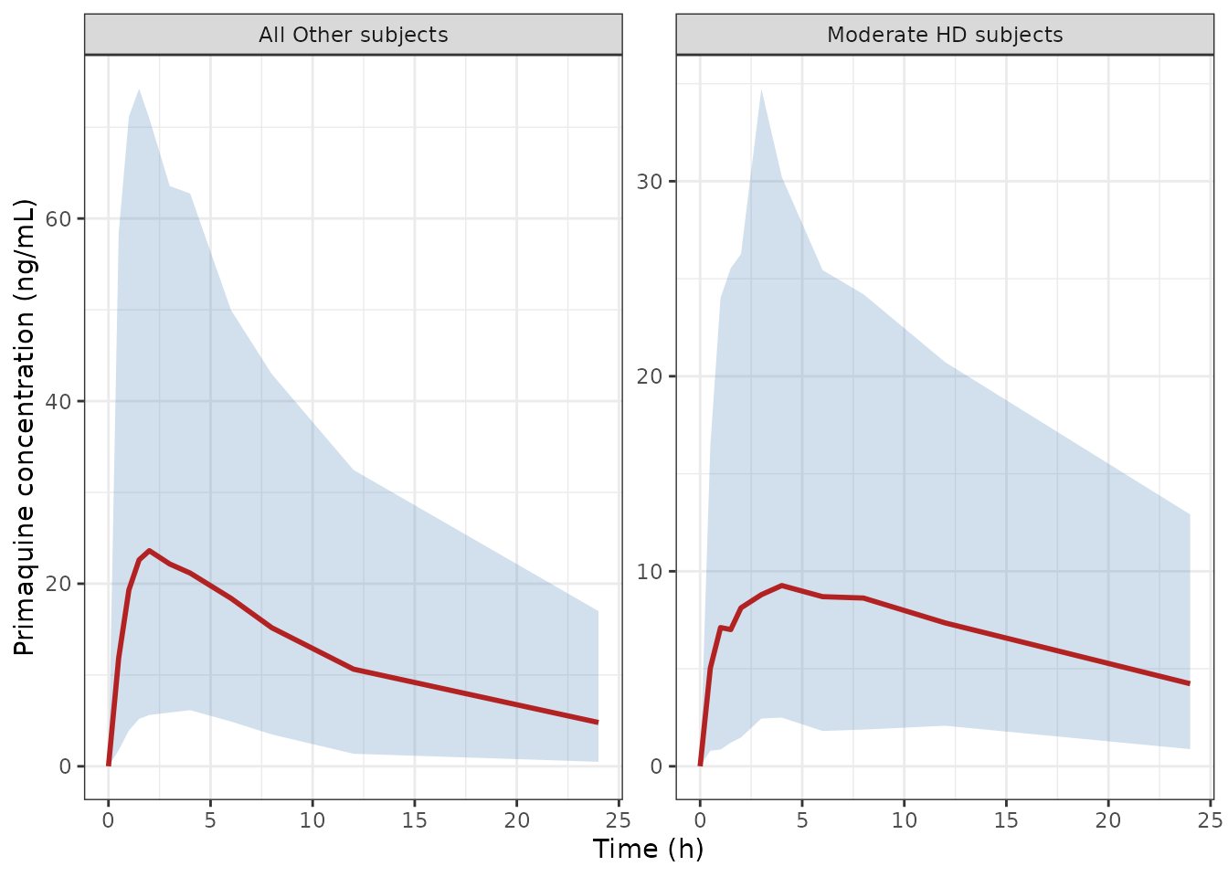

Replicates Figure 2 of Sridharan 2019: simulated concentration envelope after a single oral 15-mg dose, stratified on moderate hepatic dysfunction.

knitr::kable(
  vpc |>
    dplyr::group_by(stratum) |>
    dplyr::summarise(`Peak of median profile (ng/mL)` = round(max(mid), 1), .groups = "drop") |>
    dplyr::rename(Stratum = stratum),
  caption = "Peak of the simulated median profile by VPC stratum."
)

Peak of the simulated median profile by VPC stratum.

Stratum	Peak of median profile (ng/mL)
All Other subjects	23.6
Moderate HD subjects	9.3

The moderate-hepatic-dysfunction panel peaks roughly 2.5-fold lower than the pooled remainder, which is the qualitative separation Figure 2 shows. The separation is smaller here than the 3.3-fold seen in the typical-value profiles below because these are medians of simulated observations, where the additive residual error lifts the lower concentrations.

Replicating Figure 3 (national-guideline dosing regimens)

Figure 3 simulates typical profiles for the dosing regimens of the Indian national guidelines, side by side for “All Other Subjects” and “Moderate HD Subjects”. Because the model scales the apparent volume linearly with body weight and these regimens are specified per kilogram, the peak concentration is almost independent of the weight assumed; 70 kg is used below.

typ_profile <- function(dose_mg_per_kg, n_days, hepimp, wt = 70) {
  amt <- dose_mg_per_kg * wt * 1000 # mg/kg -> ug
  tmax_h <- 24 * n_days + 24
  ev <- dplyr::bind_rows(
    tibble::tibble(
      time = 24 * (seq_len(n_days) - 1),
      amt = amt, evid = 1L, cmt = "depot"
    ),
    tibble::tibble(
      time = seq(0, tmax_h, by = 0.25),
      amt = NA_real_, evid = 0L, cmt = "central"
    )
  ) |>
    dplyr::mutate(id = 1L, WT = wt, HEPIMP_MOD = hepimp) |>
    dplyr::arrange(time, dplyr::desc(evid)) |>
    as.data.frame()
  rxode2::rxSolve(
    mod, ev,
    omega = NA, sigma = NA, returnType = "data.frame", useLinCmt = FALSE
  ) |>
    dplyr::filter(!is.na(Cc))
}

regimens <- tibble::tribble(
  ~label,                      ~dose, ~days,
  "0.75 mg/kg single dose",     0.75,     1,
  "0.75 mg/kg/day, 14 days",    0.75,    14,
  "0.50 mg/kg/day, 14 days",    0.50,    14,
  "0.25 mg/kg/day, 14 days",    0.25,    14
)

fig3 <- dplyr::bind_rows(lapply(seq_len(nrow(regimens)), function(i) {
  r <- regimens[i, ]
  dplyr::bind_rows(
    typ_profile(r$dose, r$days, 0) |> dplyr::mutate(stratum = "All Other Subjects"),
    typ_profile(r$dose, r$days, 1) |> dplyr::mutate(stratum = "Moderate HD Subjects")
  ) |>
    dplyr::mutate(label = factor(r$label, levels = regimens$label))
}))

ggplot2::ggplot(fig3, ggplot2::aes(time, Cc, colour = stratum)) +
  ggplot2::geom_line(linewidth = 0.6) +
  ggplot2::facet_wrap(~label, scales = "free_x", ncol = 2) +
  ggplot2::labs(
    x = "Time (h)", y = "Predicted concentration (ng/mL)", colour = NULL
  ) +
  ggplot2::theme_bw() +
  ggplot2::theme(legend.position = "top")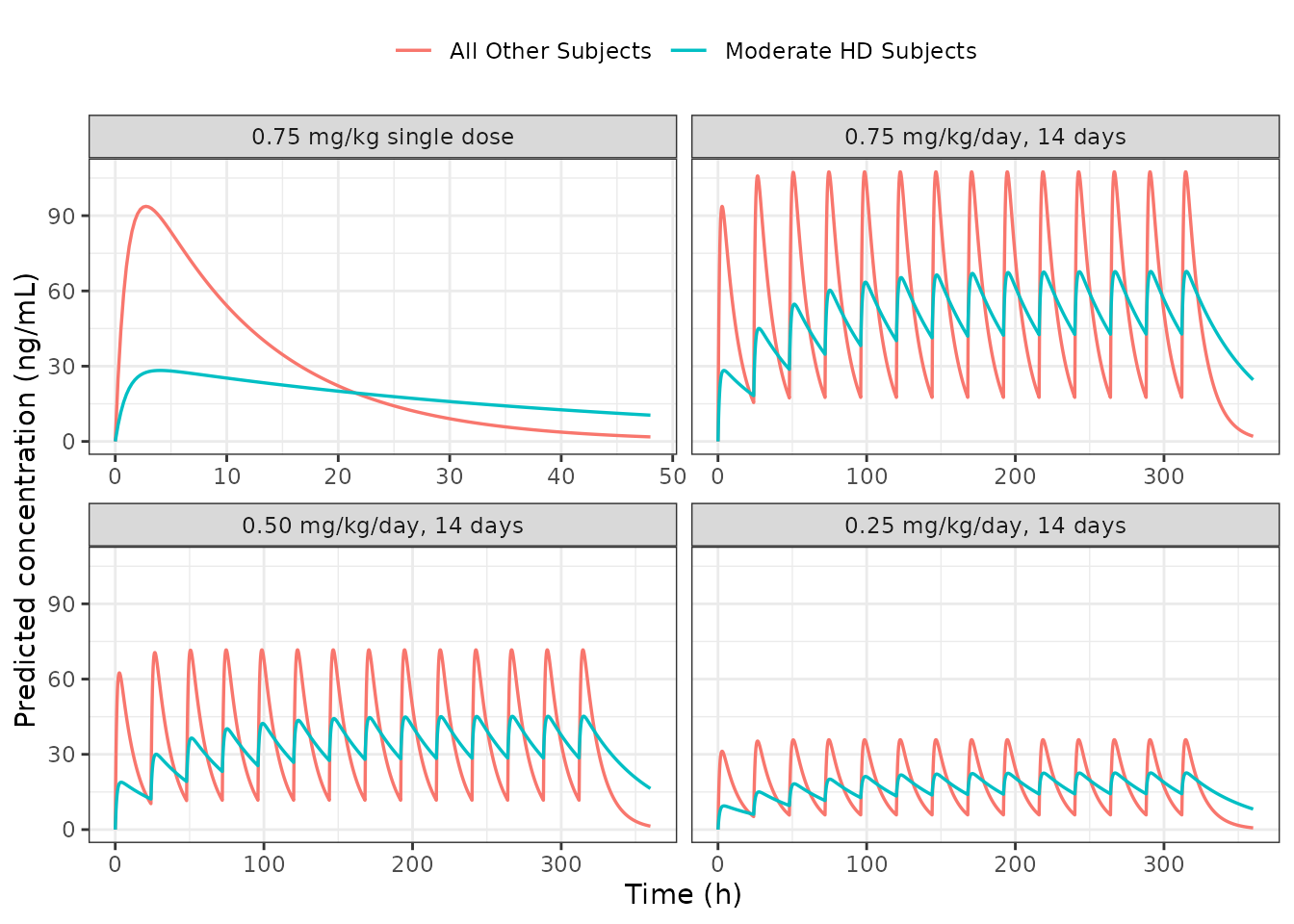

Replicates Figure 3 of Sridharan 2019: typical-value profiles for the national-guideline regimens, with and without moderate hepatic dysfunction.

Figure 3 of the source is a raster plot without printed numbers, but its single-dose panel (top row) can be read off the axes: the “All Other Subjects” peak sits just under 100 ng/mL and the “Moderate HD Subjects” peak near 30 ng/mL. Those two readings are what distinguish the two possible readings of the covariate coefficient (see Errata), so they are asserted here.

peak <- fig3 |>
  dplyr::filter(label == "0.75 mg/kg single dose") |>
  dplyr::group_by(stratum) |>
  dplyr::summarise(cmax = max(Cc), .groups = "drop")
knitr::kable(
  peak |> dplyr::rename(Stratum = stratum, `Peak (ng/mL)` = cmax),
  digits = 1,
  caption = "Typical peak after a single 0.75 mg/kg dose, against Figure 3."
)

Typical peak after a single 0.75 mg/kg dose, against Figure 3.

Stratum	Peak (ng/mL)
All Other Subjects	93.7
Moderate HD Subjects	28.3

cmax_other <- peak$cmax[peak$stratum == "All Other Subjects"]
cmax_mod <- peak$cmax[peak$stratum == "Moderate HD Subjects"]
stopifnot(
  # Read off the Figure 3 single-dose panel: a little under 100, and about 30.
  cmax_other > 85, cmax_other < 105,
  cmax_mod > 24, cmax_mod < 34,
  # The alternative reading of the covariate coefficient (a bare 2.859-fold
  # volume rather than 1 + 2.859) would put this peak at 37.3 ng/mL.
  cmax_mod < 34
)

Closed-form verification

For a one-compartment model with first-order absorption, the typical-value solution is analytic. This check compares the packaged model, solved with between-subject and residual variability switched off, against that closed form. Both sides use the same parameter values, so the only difference is numerical integration error and the bound is tight.

ka <- 0.9462
cl <- 39.14
v70 <- 438

closed_form <- function(dose_ug, wt, hepimp) {
  v <- v70 * (wt / 70) * (1 + 2.859 * hepimp)
  kel <- cl / v
  tmax <- log(ka / kel) / (ka - kel)
  cmax <- (dose_ug / v) * (ka / (ka - kel)) *
    (exp(-kel * tmax) - exp(-ka * tmax))
  c(cmax = cmax, tmax = tmax, auc = dose_ug / cl, half_life = log(2) / kel)
}

solved <- function(dose_ug, wt, hepimp) {
  ev <- dplyr::bind_rows(
    tibble::tibble(time = 0, amt = dose_ug, evid = 1L, cmt = "depot"),
    tibble::tibble(
      time = seq(0, 600, by = 0.01), amt = NA_real_, evid = 0L, cmt = "central"
    )
  ) |>
    dplyr::mutate(id = 1L, WT = wt, HEPIMP_MOD = hepimp) |>
    dplyr::arrange(time, dplyr::desc(evid)) |>
    as.data.frame()
  s <- rxode2::rxSolve(
    mod, ev,
    omega = NA, sigma = NA, returnType = "data.frame", useLinCmt = FALSE
  ) |>
    dplyr::filter(!is.na(Cc))
  i <- which.max(s$Cc)
  c(
    cmax = s$Cc[i], tmax = s$time[i],
    auc = sum(diff(s$time) * (utils::head(s$Cc, -1) + utils::tail(s$Cc, -1)) / 2),
    half_life = log(2) / (cl / (v70 * (wt / 70) * (1 + 2.859 * hepimp)))
  )
}

cf_chk <- dplyr::bind_rows(lapply(
  list(
    list(lbl = "15 mg, 70 kg, no hepatic dysfunction", wt = 70, hep = 0),
    list(lbl = "15 mg, 56 kg, moderate hepatic dysfunction", wt = 56, hep = 1)
  ),
  function(s) {
    a <- closed_form(dose_ug, s$wt, s$hep)
    b <- solved(dose_ug, s$wt, s$hep)
    tibble::tibble(
      Scenario = s$lbl,
      Quantity = c("Cmax (ng/mL)", "Tmax (h)", "AUC0-inf (ng*h/mL)", "t1/2 (h)"),
      `Closed form` = as.numeric(a),
      `rxode2` = as.numeric(b)
    )
  }
)) |>
  dplyr::mutate(`% diff` = 100 * (rxode2 - `Closed form`) / `Closed form`)

knitr::kable(cf_chk, digits = c(0, 0, 3, 3, 3), caption = "Packaged model against the analytic one-compartment oral solution.")

Packaged model against the analytic one-compartment oral solution.

Scenario	Quantity	Closed form	rxode2	% diff
15 mg, 70 kg, no hepatic dysfunction	Cmax (ng/mL)	26.775	26.775	0.000
15 mg, 70 kg, no hepatic dysfunction	Tmax (h)	2.754	2.750	-0.147
15 mg, 70 kg, no hepatic dysfunction	AUC0-inf (ng*h/mL)	383.240	383.239	0.000
15 mg, 70 kg, no hepatic dysfunction	t1/2 (h)	7.757	7.757	0.000
15 mg, 56 kg, moderate hepatic dysfunction	Cmax (ng/mL)	9.937	9.937	0.000
15 mg, 56 kg, moderate hepatic dysfunction	Tmax (h)	3.802	3.800	-0.042
15 mg, 56 kg, moderate hepatic dysfunction	AUC0-inf (ng*h/mL)	383.240	383.240	0.000
15 mg, 56 kg, moderate hepatic dysfunction	t1/2 (h)	23.947	23.947	0.000

stopifnot(
  # Same parameters on both sides: this is pure integration error.
  max(abs(cf_chk$`% diff`[cf_chk$Quantity != "Tmax (h)"])) < 0.5,
  # Tmax is resolved only to the 0.01 h observation grid.
  max(abs(cf_chk$rxode2[cf_chk$Quantity == "Tmax (h)"] -
    cf_chk$`Closed form`[cf_chk$Quantity == "Tmax (h)"])) < 0.02
)

The moderate-hepatic-dysfunction row also pins the covariate arithmetic: the apparent volume is multiplied by 1 + 2.859 = 3.859, which lengthens the terminal half-life from 7.8 h to 29.9 h at a fixed clearance.

PKNCA validation

Non-compartmental analysis is run on the simulated study using the same design the paper analysed – a single 15-mg oral dose sampled at 11 nominal times – so that the trapezoidal and extrapolation behaviour of NCA applies equally to both sides of the comparison.

sim_nca <- sim |>
  dplyr::filter(!is.na(Cobs)) |>
  dplyr::select(id, time, Cobs, group)

dose_df <- events |>
  dplyr::filter(evid == 1) |>
  dplyr::select(id, time, amt, group) |>
  dplyr::mutate(amt = amt / 1000) # ug -> mg, to match the published dose unit

conc_obj <- PKNCA::PKNCAconc(
  sim_nca, Cobs ~ time | group + id,
  concu = "ng/mL", timeu = "h"
)
dose_obj <- PKNCA::PKNCAdose(
  dose_df, amt ~ time | group + id,
  doseu = "mg"
)

intervals <- data.frame(
  start = 0,
  end = Inf,
  cmax = TRUE,
  tmax = TRUE,
  aucinf.obs = TRUE,
  half.life = TRUE
)

nca_res <- PKNCA::pk.nca(
  PKNCA::PKNCAdata(conc_obj, dose_obj, intervals = intervals)
)
#> Warning: Too few points for half-life calculation (min.hl.points=3 with only 2 points)
#> Too few points for half-life calculation (min.hl.points=3 with only 2 points)
#> Warning: Too few points for half-life calculation (min.hl.points=3 with only 1 points)
#> Too few points for half-life calculation (min.hl.points=3 with only 1 points)
#> Too few points for half-life calculation (min.hl.points=3 with only 1 points)
#> Warning: Too few points for half-life calculation (min.hl.points=3 with only 2
#> points)
#> Warning: Too few points for half-life calculation (min.hl.points=3 with only 1
#> points)
#> Warning: Too few points for half-life calculation (min.hl.points=3 with only 2 points)
#> Too few points for half-life calculation (min.hl.points=3 with only 2 points)
#> Too few points for half-life calculation (min.hl.points=3 with only 2 points)
#> Warning: Too few points for half-life calculation (min.hl.points=3 with only 0
#> points)
#> Warning: Too few points for half-life calculation (min.hl.points=3 with only 2 points)
#> Too few points for half-life calculation (min.hl.points=3 with only 2 points)
#> Warning: Too few points for half-life calculation (min.hl.points=3 with only 0
#> points)
#> Warning: Too few points for half-life calculation (min.hl.points=3 with only 2 points)
#> Too few points for half-life calculation (min.hl.points=3 with only 2 points)
#> Too few points for half-life calculation (min.hl.points=3 with only 2 points)
#> Too few points for half-life calculation (min.hl.points=3 with only 2 points)
#> Warning: Too few points for half-life calculation (min.hl.points=3 with only 0
#> points)
#> Warning: Too few points for half-life calculation (min.hl.points=3 with only 2 points)
#> Too few points for half-life calculation (min.hl.points=3 with only 2 points)
#> Too few points for half-life calculation (min.hl.points=3 with only 2 points)
#> Too few points for half-life calculation (min.hl.points=3 with only 2 points)
#> Too few points for half-life calculation (min.hl.points=3 with only 2 points)
#> Too few points for half-life calculation (min.hl.points=3 with only 2 points)
#> Too few points for half-life calculation (min.hl.points=3 with only 2 points)
#> Too few points for half-life calculation (min.hl.points=3 with only 2 points)
#> Too few points for half-life calculation (min.hl.points=3 with only 2 points)
#> Warning: Too few points for half-life calculation (min.hl.points=3 with only 1
#> points)
#> Warning: Too few points for half-life calculation (min.hl.points=3 with only 2 points)
#> Too few points for half-life calculation (min.hl.points=3 with only 2 points)
#> Too few points for half-life calculation (min.hl.points=3 with only 2 points)
#> Warning: Too few points for half-life calculation (min.hl.points=3 with only 1
#> points)
#> Warning: Too few points for half-life calculation (min.hl.points=3 with only 2 points)
#> Too few points for half-life calculation (min.hl.points=3 with only 2 points)
#> Too few points for half-life calculation (min.hl.points=3 with only 2 points)
#> Too few points for half-life calculation (min.hl.points=3 with only 2 points)
#> Warning: Too few points for half-life calculation (min.hl.points=3 with only 1 points)
#> Too few points for half-life calculation (min.hl.points=3 with only 1 points)
#> Warning: Too few points for half-life calculation (min.hl.points=3 with only 2 points)
#> Too few points for half-life calculation (min.hl.points=3 with only 2 points)
#> Warning: Too few points for half-life calculation (min.hl.points=3 with only 1 points)
#> Too few points for half-life calculation (min.hl.points=3 with only 1 points)
#> Too few points for half-life calculation (min.hl.points=3 with only 1 points)
#> Too few points for half-life calculation (min.hl.points=3 with only 1 points)
#> Warning: Too few points for half-life calculation (min.hl.points=3 with only 2 points)
#> Too few points for half-life calculation (min.hl.points=3 with only 2 points)
#> Warning: Too few points for half-life calculation (min.hl.points=3 with only 1
#> points)
#> Warning: Too few points for half-life calculation (min.hl.points=3 with only 2 points)
#> Too few points for half-life calculation (min.hl.points=3 with only 2 points)
#> Warning: Too few points for half-life calculation (min.hl.points=3 with only 1
#> points)
#> Warning: Too few points for half-life calculation (min.hl.points=3 with only 2 points)
#> Too few points for half-life calculation (min.hl.points=3 with only 2 points)
#> Too few points for half-life calculation (min.hl.points=3 with only 2 points)
#> Warning: Too few points for half-life calculation (min.hl.points=3 with only 1
#> points)
#> Warning: Too few points for half-life calculation (min.hl.points=3 with only 2
#> points)
#> Warning: Too few points for half-life calculation (min.hl.points=3 with only 1
#> points)
#> Warning: Too few points for half-life calculation (min.hl.points=3 with only 2 points)
#> Too few points for half-life calculation (min.hl.points=3 with only 2 points)
#> Warning: Too few points for half-life calculation (min.hl.points=3 with only 0
#> points)
#> Warning: Too few points for half-life calculation (min.hl.points=3 with only 1 points)
#> Too few points for half-life calculation (min.hl.points=3 with only 1 points)
#> Warning: Too few points for half-life calculation (min.hl.points=3 with only 2
#> points)
#> Warning: Too few points for half-life calculation (min.hl.points=3 with only 0
#> points)
#> Warning: Too few points for half-life calculation (min.hl.points=3 with only 2
#> points)
#> Warning: Too few points for half-life calculation (min.hl.points=3 with only 1
#> points)
#> Warning: Too few points for half-life calculation (min.hl.points=3 with only 2 points)
#> Too few points for half-life calculation (min.hl.points=3 with only 2 points)
#> Warning: Too few points for half-life calculation (min.hl.points=3 with only 1 points)
#> Too few points for half-life calculation (min.hl.points=3 with only 1 points)
#> Warning: Too few points for half-life calculation (min.hl.points=3 with only 2
#> points)
#> Warning: Too few points for half-life calculation (min.hl.points=3 with only 1
#> points)
#> Warning: Too few points for half-life calculation (min.hl.points=3 with only 0
#> points)
#> Warning: Too few points for half-life calculation (min.hl.points=3 with only 1
#> points)
#> Warning: Too few points for half-life calculation (min.hl.points=3 with only 2
#> points)
#> Warning: Too few points for half-life calculation (min.hl.points=3 with only 1 points)
#> Too few points for half-life calculation (min.hl.points=3 with only 1 points)
#> Too few points for half-life calculation (min.hl.points=3 with only 1 points)
#> Too few points for half-life calculation (min.hl.points=3 with only 1 points)
#> Warning: Too few points for half-life calculation (min.hl.points=3 with only 2
#> points)
#> Warning: Too few points for half-life calculation (min.hl.points=3 with only 0
#> points)
#> Warning: Too few points for half-life calculation (min.hl.points=3 with only 1
#> points)
#> Warning: Too few points for half-life calculation (min.hl.points=3 with only 2 points)
#> Too few points for half-life calculation (min.hl.points=3 with only 2 points)
#> Too few points for half-life calculation (min.hl.points=3 with only 2 points)
#> Too few points for half-life calculation (min.hl.points=3 with only 2 points)
#> Too few points for half-life calculation (min.hl.points=3 with only 2 points)
#> Too few points for half-life calculation (min.hl.points=3 with only 2 points)
#> Too few points for half-life calculation (min.hl.points=3 with only 2 points)
#> Warning: Too few points for half-life calculation (min.hl.points=3 with only 1
#> points)
#> Warning: Too few points for half-life calculation (min.hl.points=3 with only 2 points)
#> Too few points for half-life calculation (min.hl.points=3 with only 2 points)
#> Too few points for half-life calculation (min.hl.points=3 with only 2 points)
#> Too few points for half-life calculation (min.hl.points=3 with only 2 points)
#> Too few points for half-life calculation (min.hl.points=3 with only 2 points)
#> Too few points for half-life calculation (min.hl.points=3 with only 2 points)
#> Warning: Too few points for half-life calculation (min.hl.points=3 with only 0
#> points)
#> Warning: Too few points for half-life calculation (min.hl.points=3 with only 2
#> points)
#> Warning: Too few points for half-life calculation (min.hl.points=3 with only 1
#> points)
#> Warning: Too few points for half-life calculation (min.hl.points=3 with only 2
#> points)
#> Warning: Too few points for half-life calculation (min.hl.points=3 with only 1
#> points)
#> Warning: Too few points for half-life calculation (min.hl.points=3 with only 2
#> points)

Comparison against the published NCA

Table 1 of the source reports median (range) NCA parameters per stratum. The comparison below uses those medians as the reference.

published <- tibble::tribble(
  ~group,                          ~cmax, ~tmax, ~aucinf.obs, ~half.life,
  "Healthy",                        29.3,   3.0,       314.1,        4.1,
  "Mild hepatic dysfunction",       45.6,   3.0,       303.0,        6.6,
  "Moderate hepatic dysfunction",   14.4,   3.5,       117.2,        4.3,
  "Renal dysfunction",              45.6,   2.0,       261.9,        3.5
)

cmp <- nlmixr2lib::ncaComparisonTable(
  simulated = nca_res,
  reference = published,
  by = "group",
  units = c(
    cmax = "ng/mL", tmax = "h",
    aucinf.obs = "ng*h/mL", half.life = "h"
  ),
  tolerance_pct = 20
)

knitr::kable(
  cmp,
  caption = paste(
    "Simulated versus published NCA (Table 1 medians).",
    "* differs from the reference by more than 20%."
  ),
  align = c("l", "l", "r", "r", "r")
)

Simulated versus published NCA (Table 1 medians). * differs from the reference by more than 20%.

NCA parameter	group	Reference	Simulated	% diff
Cmax (ng/mL)	Healthy	29.3	29.2	-0.2%
Cmax (ng/mL)	Mild hepatic dysfunction	45.6	33.4	-26.8%*
Cmax (ng/mL)	Moderate hepatic dysfunction	14.4	13	-9.8%
Cmax (ng/mL)	Renal dysfunction	45.6	39.6	-13.1%
Tmax (h)	Healthy	3	3	+0.0%
Tmax (h)	Mild hepatic dysfunction	3	2	-33.3%*
Tmax (h)	Moderate hepatic dysfunction	3.5	3	-14.3%
Tmax (h)	Renal dysfunction	2	2	+0.0%
AUC0-∞ (obs) (ng*h/mL)	Healthy	314	378	+20.5%*
AUC0-∞ (obs) (ng*h/mL)	Mild hepatic dysfunction	303	391	+29.0%*
AUC0-∞ (obs) (ng*h/mL)	Moderate hepatic dysfunction	117	309	+163.3%*
AUC0-∞ (obs) (ng*h/mL)	Renal dysfunction	262	339	+29.6%*
t½ (h)	Healthy	4.1	8	+95.1%*
t½ (h)	Mild hepatic dysfunction	6.6	6.74	+2.1%
t½ (h)	Moderate hepatic dysfunction	4.3	13	+201.2%*
t½ (h)	Renal dysfunction	3.5	5.75	+64.4%*

attr(cmp, "footnote")
#> [1] "* differs from reference by more than ±20%."

chk <- cmp |>
  dplyr::mutate(
    parameter = cmp[[1]],
    pct = suppressWarnings(as.numeric(gsub("[^0-9.eE+-]", "", `% diff`)))
  )
cmax_pct <- chk$pct[grepl("^Cmax", chk$parameter)]
tmax_pct <- chk$pct[grepl("^Tmax", chk$parameter)]

stopifnot(
  # Structural gate on the exposure the model does reproduce. A mis-transcribed
  # dose, volume or covariate multiplier moves peak concentration by a factor,
  # not by tens of percent, so a centre statistic over the four strata catches
  # it with room to spare for the sampling noise of a 200-subject median.
  length(cmax_pct) == 4L,
  stats::median(abs(cmax_pct), na.rm = TRUE) < 30,
  max(abs(cmax_pct), na.rm = TRUE) < 45,
  # Tmax depends on ka and on kel, so it also moves if either is wrong, but it
  # is resolved only to the paper's coarse nominal sampling grid.
  stats::median(abs(tmax_pct), na.rm = TRUE) < 30
)

Peak exposure is reproduced in all four strata. Median simulated Cmax lands within 27% of the published median everywhere and within 10% in the healthy and moderate-hepatic-dysfunction strata, and Tmax matches the published median exactly in three of the four. That is the comparison most sensitive to a mis-transcribed dose, apparent volume, or hepatic covariate multiplier, and it is the one asserted above.

AUC and terminal half-life are systematically over-predicted, and this is a property of the published model rather than of the packaged implementation. Two distinct effects are visible in the table:

• In the healthy, mild-hepatic-dysfunction and renal-dysfunction strata, simulated AUC0-inf runs 20-30% above the published medians and half-life runs up to 95% above them. The model’s typical clearance, 39.14 L/h, is lower than the median apparent clearance Table 1 reports for every one of those strata (45.6, 50.95 and 60.4 L/h), and a lower clearance at a fixed volume produces both a larger AUC and a longer terminal slope. The two sides of the comparison are not independent estimates of the same quantity: Table 1’s values are medians of individually-derived NCA on 11 samples per subject, while the model is a population fit to the same records, and the paper itself publishes both without reconciling them.
• The moderate-hepatic-dysfunction stratum diverges much further, at +163% on AUC and +201% on half-life. Table 1’s own NCA shows that group with both an approximately threefold higher apparent volume (886.71 versus 300.7 L) and an approximately fourfold higher apparent clearance (183.71 versus 45.6 L/h) – the signature of reduced bioavailability, since CL/F and V/F both scale as 1/F. The final population model attributes the entire effect to volume and leaves clearance untouched, so it necessarily predicts an unchanged AUC and a terminal half-life stretched from 7.8 h to 29.9 h, where the observed group had a median half-life of 4.3 h and roughly a third of the healthy group’s AUC. The authors reach the same diagnosis in the Discussion: “We hypothesize that presence of a gut wall edema may hamper the absorption of the drug in these patients leading to reduced bioavailability.”

No parameter has been tuned to close either gap. Users simulating total exposure in moderate hepatic dysfunction with this model should be aware that its AUC and half-life predictions for that stratum are not supported by the source paper’s own non-compartmental analysis.

Assumptions and deviations

• Dosing unit. The model’s dosing unit is micrograms so that amounts over volumes in litres give ng/mL directly, the unit in which Table 1, Table 2 and the additive residual error are all reported. A 15-mg dose is therefore entered as amt = 15000.
• Dose is 15 mg as administered. The paper describes both a “single-dose (15 mg) PQ” and a “Tablet PQ phosphate 15-mg” and does not state whether the 15 mg is base or phosphate salt. Simulating 15 mg reproduces the paper’s own Table 1 peak concentrations and Figure 3 panels; simulating the 8.6-mg base equivalent of a 15-mg phosphate tablet would not. The parameters are apparent (CL/F, V/F) and are consistent only with the dose amount the authors themselves entered.
• Weight exponent on volume. The paper states that volume was “normalized to 70-kg person” in all models but never prints an exponent. e_wt_vc is held at 1, the linear scaling that a plain normalization denotes, rather than estimated. No weight scaling is applied to clearance, which the paper’s covariate search did not retain.
• Between-subject variability convention. Table 2 publishes the etas as “% CV”. The same column header is used for the proportional residual error, where it can only mean 100 x sqrt(variance), so the etas are read on that convention and each variance is (%CV/100)^2. Reading them instead as log-normal CVs, log(1 + CV^2), would give 0.353 / 0.367 / 0.470 in place of 0.424 / 0.443 / 0.600. The paper gives no footnote to settle it.
• Bioavailability. F is never estimated, so every clearance and volume in the model is apparent. No lfdepot is carried.
• Flip-flop constraint. The estimation constrained Ka above the elimination rate constant. At the published estimates the constraint is inactive (Ka = 0.946/h against kel = 0.089/h at 70 kg), so it is not encoded in the model; it would only matter when refitting.
• Sex. sex_female_pct is left NA because the paper reports sex only as per-group male:female ratios (5:1, 5:1, all male, 2:1) that do not resolve to integer counts for the 12- and 22-subject groups.
• Simulated cohort size. 200 subjects per stratum are simulated rather than the 13 / 12 / 6 / 22 enrolled, so that the medians compared against Table 1 are stable across machines. Covariate distributions match Table 1.
• BLQ handling. Simulated concentrations that fall below zero once the additive residual error is applied are dropped before NCA; the paper does not report an assay lower limit of quantification.

Errata and internal inconsistencies in the source

The source is internally inconsistent in four places. In each case the value used in the model is the one supported by Table 2, the Results text and the paper’s own figures, over the Abstract.

1. Volume of distribution. The Abstract reports the final V as 498 L; the Results text (“volume of distribution (Vd) was 438 L”) and Table 2 (V theta = 438, bootstrap median 439.6, 95% CI 345.37-550.53) both give 438 L. 438 L is used, and it is the value that reproduces Figure 3.
2. Proportional residual error. The Abstract reports “proportion error 12% CV”; Table 2 reports 32.06% CV with a bootstrap 95% CI of 27.98-35.74, which excludes 12%. 32.06% is used.
3. Which hepatic stratum is significant. The Abstract says “Mild hepatic dysfunction was a significant covariate on volume of distribution”; the Results (“Only the moderate hepatic dysfunction showed to be significant on the volume of distribution”), the Table 2 row label (“Moderate HD on V”), the Conclusion and both figures all say moderate. Moderate is used, and mild hepatic dysfunction is recorded in covariatesDataExcluded.
4. Residual-error equation subscripts. Methods Equation 2 is printed as Cij = C'ij (1 + eps_add,j) + eps_prop,j, which transposes the two error terms: the multiplicative term is labelled additive and the standalone term proportional. Table 2’s units settle the orientation, since the additive term carries ng/mL and the proportional term % CV. The model uses the conventional orientation, C * (1 + eps_prop) + eps_add.

Two further points of reading:

• Magnitude of the hepatic covariate effect. The Methods covariate function is proportional, TVP = P x (1 + theta_mild x FLAG) x (1 + theta_mod x FLAG1), so theta_mod = 2.859 is a fractional increase and the multiplier on volume is 1 + 2.859 = 3.859. The prose (“the parameter increased approximately three folds”) reads naturally either as that fractional increase or as a bare 2.859-fold multiplier. Figure 3 settles it: at 0.75 mg/kg as a single dose it shows peaks near 95 and 30 ng/mL for the two strata, which the 3.859-fold volume reproduces (93.7 and 28.3 ng/mL) and a bare 2.859-fold volume does not (93.7 and 37.3 ng/mL). This is asserted in the Figure 3 section above.
• Additive-error RSE. The Results text gives the additive residual variability RSE as 116%; Table 2 gives 102.5%. Neither enters the model.

Session information

sessionInfo()
#> R version 4.6.1 (2026-06-24)
#> Platform: x86_64-pc-linux-gnu
#> Running under: Ubuntu 24.04.5 LTS
#> 
#> Matrix products: default
#> BLAS:   /usr/lib/x86_64-linux-gnu/openblas-pthread/libblas.so.3 
#> LAPACK: /usr/lib/x86_64-linux-gnu/openblas-pthread/libopenblasp-r0.3.26.so;  LAPACK version 3.12.0
#> 
#> locale:
#>  [1] LC_CTYPE=C.UTF-8       LC_NUMERIC=C           LC_TIME=C.UTF-8       
#>  [4] LC_COLLATE=C.UTF-8     LC_MONETARY=C.UTF-8    LC_MESSAGES=C.UTF-8   
#>  [7] LC_PAPER=C.UTF-8       LC_NAME=C              LC_ADDRESS=C          
#> [10] LC_TELEPHONE=C         LC_MEASUREMENT=C.UTF-8 LC_IDENTIFICATION=C   
#> 
#> time zone: UTC
#> tzcode source: system (glibc)
#> 
#> attached base packages:
#> [1] stats     graphics  grDevices utils     datasets  methods   base     
#> 
#> other attached packages:
#> [1] ggplot2_4.0.3         tidyr_1.3.2           dplyr_1.2.1          
#> [4] rxode2_5.1.8          PKNCA_0.12.1          nlmixr2lib_0.3.2.9000
#> 
#> loaded via a namespace (and not attached):
#>  [1] gtable_0.3.6        xfun_0.61           bslib_0.12.0       
#>  [4] rxode2lincmt_0.1.0  lattice_0.22-9      vctrs_0.7.3        
#>  [7] tools_4.6.1         generics_0.1.4      parallel_4.6.1     
#> [10] tibble_3.3.1        symengine_0.2.13    pkgconfig_2.0.3    
#> [13] data.table_1.18.6.1 checkmate_2.3.4     RColorBrewer_1.1-3 
#> [16] S7_0.2.2            desc_1.4.3          lifecycle_1.0.5    
#> [19] compiler_4.6.1      farver_2.1.2        textshaping_1.0.5  
#> [22] fontawesome_0.5.3   htmltools_0.5.9     sys_3.4.3          
#> [25] sass_0.4.10         yaml_2.3.12         pillar_1.11.1      
#> [28] pkgdown_2.2.1       crayon_1.5.3        jquerylib_0.1.4    
#> [31] whisker_0.4.1       openssl_2.4.2       cachem_1.1.0       
#> [34] nlme_3.1-169        tidyselect_1.2.1    digest_0.6.39      
#> [37] lotri_1.0.5         purrr_1.2.2         labeling_0.4.3     
#> [40] rxode2ll_2.0.18     fastmap_1.2.0       grid_4.6.1         
#> [43] cli_3.6.6           dparser_1.3.1-13    magrittr_2.0.5     
#> [46] withr_3.0.3         scales_1.4.0        backports_1.5.1    
#> [49] rmarkdown_2.32      otel_0.2.0          askpass_1.2.1      
#> [52] ragg_1.5.2          memoise_2.0.1       evaluate_1.0.5     
#> [55] knitr_1.52          rex_1.2.2           PreciseSums_0.7    
#> [58] rlang_1.3.0         downlit_0.4.5       Rcpp_1.1.2         
#> [61] glue_1.8.1          xml2_1.6.0          jsonlite_2.0.0     
#> [64] R6_2.6.1            systemfonts_1.3.2   fs_2.1.0