COX-2 selective inhibitors celecoxib, mavacoxib and meloxicam in cockatiels (Dhondt 2017)
Source:vignettes/articles/Dhondt_2017_cox2inhibitors_cockatiel.Rmd
Dhondt_2017_cox2inhibitors_cockatiel.RmdModel and source
Dhondt and colleagues gave three COX-2 selective non-steroidal anti-inflammatory drugs to cockatiels (Nymphicus hollandicus) and fitted a population PK model to each route and formulation separately. Celecoxib and mavacoxib were each given intravenously as an analytical standard solution (STD), orally as that same standard solution, and orally as the ground commercial tablet (CF); meloxicam, for which an injectable commercial formulation exists, was given intravenously and orally as the commercial product only. That is eight independent fits, reported in Tables 1, 2 and 3, and they are packaged here as eight model files.
The fits share no parameters. The oral arms report apparent
disposition (Vd/F, Cl/F) because no
bioavailability term was estimated, so the oral Vd/F is not
the intravenous Vd rescaled by the separately reported
F% (celecoxib STD: 5.87 L/kg oral against 4.67 L/kg
intravenous at F = 110%). Collapsing the arms into one model per drug
would therefore not reproduce either profile, which is why each arm is
its own file.
arms <- tibble::tribble(
  ~arm,                   ~drug,        ~model,                                       ~dose, ~dose_cmt,
  "celecoxib i.v. STD",   "celecoxib",  "Dhondt_2017_celecoxib_cockatiel_iv",         10000, "central",
  "celecoxib oral STD",   "celecoxib",  "Dhondt_2017_celecoxib_cockatiel_oral_std",   10000, "depot",
  "celecoxib oral CF",    "celecoxib",  "Dhondt_2017_celecoxib_cockatiel_oral_cf",    10000, "depot",
  "mavacoxib i.v. STD",   "mavacoxib",  "Dhondt_2017_mavacoxib_cockatiel_iv",          4000, "central",
  "mavacoxib oral STD",   "mavacoxib",  "Dhondt_2017_mavacoxib_cockatiel_oral_std",    4000, "depot",
  "mavacoxib oral CF",    "mavacoxib",  "Dhondt_2017_mavacoxib_cockatiel_oral_cf",     4000, "depot",
  "meloxicam i.v.",       "meloxicam",  "Dhondt_2017_meloxicam_cockatiel_iv",          1000, "central",
  "meloxicam oral",       "meloxicam",  "Dhondt_2017_meloxicam_cockatiel_oral",        1000, "depot"
)

mods <- stats::setNames(lapply(arms$model, readModelDb), arms$arm)
uis <- lapply(mods, rxode2::rxode)
#> ℹ parameter labels from comments will be replaced by 'label()'
#> ℹ parameter labels from comments will be replaced by 'label()'
#> ℹ parameter labels from comments will be replaced by 'label()'
#> ℹ parameter labels from comments will be replaced by 'label()'
#> ℹ parameter labels from comments will be replaced by 'label()'
#> ℹ parameter labels from comments will be replaced by 'label()'
#> ℹ parameter labels from comments will be replaced by 'label()'
#> ℹ parameter labels from comments will be replaced by 'label()'

knitr::kable(
  arms |>
    dplyr::mutate(`Dose (mg/kg)` = dose / 1000) |>
    dplyr::select(arm, model, `Dose (mg/kg)`, dose_cmt) |>
    dplyr::rename(
      "Arm" = arm,
      "Model file" = model,
      "Dosed compartment" = dose_cmt
    ),
  caption = "The eight independently fitted arms of Dhondt 2017."
)| Arm | Model file | Dose (mg/kg) | Dosed compartment |
|---|---|---|---|
| celecoxib i.v. STD | Dhondt_2017_celecoxib_cockatiel_iv | 10 | central |
| celecoxib oral STD | Dhondt_2017_celecoxib_cockatiel_oral_std | 10 | depot |
| celecoxib oral CF | Dhondt_2017_celecoxib_cockatiel_oral_cf | 10 | depot |
| mavacoxib i.v. STD | Dhondt_2017_mavacoxib_cockatiel_iv | 4 | central |
| mavacoxib oral STD | Dhondt_2017_mavacoxib_cockatiel_oral_std | 4 | depot |
| mavacoxib oral CF | Dhondt_2017_mavacoxib_cockatiel_oral_cf | 4 | depot |
| meloxicam i.v. | Dhondt_2017_meloxicam_cockatiel_iv | 1 | central |
| meloxicam oral | Dhondt_2017_meloxicam_cockatiel_oral | 1 | depot |
- Citation: Dhondt L, Devreese M, Croubels S, De Baere S, Haesendonck R, Goessens T, Gehring R, De Backer P, Antonissen G. Comparative population pharmacokinetics and absolute oral bioavailability of COX-2 selective inhibitors celecoxib, mavacoxib and meloxicam in cockatiels (Nymphicus hollandicus). Sci Rep. 2017;7(1):12043. doi:10.1038/s41598-017-12159-z.
- Article: https://doi.org/10.1038/s41598-017-12159-z
Example description (the intravenous celecoxib arm):
Preclinical (cockatiel). One-compartment population PK model with first-order elimination for celecoxib after a single 10 mg/kg intravenous bolus of an analytical standard solution (STD) to cockatiels (Nymphicus hollandicus). Fitted in Phoenix NLME (FOCE-ELS) as the intravenous arm of a three-drug comparative study; Table 1, ‘IV STD’ block. Every volume and clearance term in the source is normalised to body weight, so the model is coded per kilogram: the dosed amount is ug/kg and the volume is L/kg, which makes central/vc land directly in ng/mL, the assay units of Figure 2a. Body weight and sex were screened as covariates and neither was retained. See Dhondt_2017_celecoxib_cockatiel_oral_std and Dhondt_2017_celecoxib_cockatiel_oral_cf for the separately fitted oral arms.
Population
Ninety cockatiels (45 male / 45 female), 6-12 months old, were group-housed in an aviary at Ghent University and randomly allocated by sex to the experimental groups; each bird took part in at least one and at most two of the three drug studies, with one to six months of washout and recovery between experiments (Methods, “Animals and experimental procedure”).
Celecoxib (10 mg/kg) was given to 22 birds (11/11, 93 +/- 10 g) as the ground commercial tablet orally, and to a separate 34 birds (17/17, 91 +/- 10 g) as the standard solution both orally and intravenously in a two-way crossover with one month of washout. Mavacoxib (4 mg/kg) went to 26 birds (13/13, 93 +/- 9 g) as the commercial tablet orally, and to 40 birds (20/20, 101 +/- 8 g) as the standard solution in a two-way crossover with three months of washout. Meloxicam (1 mg/kg) went to 24 birds (12/12, 101 +/- 12 g) in a two-way crossover with one month between administrations.
Cockatiels yield very little blood, so a sparse sampling protocol was used: sampling times were randomly allocated across birds, with a maximum of two samples per bird for celecoxib and meloxicam and three for mavacoxib. It is that sparseness that made the non-linear mixed-effects approach necessary. All three drugs were quantified in plasma by LC-MS/MS; the limit of quantification was 5 ng/mL for the two coxibs and 10 ng/mL for meloxicam, and values below it were dropped before fitting. Feed was withheld from 8 h before until 4 h after dosing, but every bird received a 2 mL intra-crop feed bolus immediately after dosing, because food is known to raise the oral bioavailability of both coxibs in dogs.
Plasma protein binding was measured separately and exceeded 95% for all three drugs (celecoxib 98.98 +/- 0.07%, mavacoxib 97.02 +/- 0.32%, meloxicam 95.02 +/- 0.01%). It is not a model parameter and is recorded only in the model metadata.
str(uis[["meloxicam i.v."]]$population)
#> List of 11
#>  $ species       : chr "cockatiel (Nymphicus hollandicus)"
#>  $ n_subjects    : int 24
#>  $ n_studies     : int 1
#>  $ age_range     : chr "6-12 months"
#>  $ weight_median : chr "101 g"
#>  $ weight_range  : chr "101 +/- 12 g (mean +/- SD)"
#>  $ sex_female_pct: num 50
#>  $ disease_state : chr "Healthy (no disease model)"
#>  $ dose_range    : chr "Single 1 mg/kg body weight intravenous bolus into the vena cutanea ulnaris (wing vein) of the commercial inject"| __truncated__
#>  $ regions       : chr "Belgium (Ghent University, Merelbeke)"
#>  $ notes         : chr "The 24 birds (12 male / 12 female) received meloxicam both intravenously and orally in a two-way crossover with"| __truncated__
Source trace
Per-parameter provenance is recorded as an in-file comment beside
each ini() entry in the eight files under
inst/modeldb/specificDrugs/. The table below collects
them.
| Parameter | celecoxib i.v. | celecoxib oral STD | celecoxib oral CF | Source |
|---|---|---|---|---|
lvc (Vd or Vd/F, L/kg) |
4.67 | 5.87 | 5.49 | Table 1 |
lcl (Cl or Cl/F, L/h/kg) |
2.42 | 2.19 | 4.32 | Table 1 |
lka (1/h) |
n/a | 0.27 | 0.39 | Table 1 |
ltlag (h) |
n/a | n/a | 0.33 | Table 1 |
etalvc (omega) |
< 0.001 | 0.948 | < 0.001 | Table 1, omega column |
etalcl (omega) |
0.0418 | 0.707 | 0.055 | Table 1, omega column |
etalka (omega) |
n/a | 0.063 | < 0.001 | Table 1, omega column |
etaltlag (omega) |
n/a | n/a | 0.207 | Table 1, omega column |
| residual |
prop 0.42 |
add 8.02 |
add 15.18 + prop 0.41 |
Table 1 |
| Parameter | mavacoxib i.v. | mavacoxib oral STD | mavacoxib oral CF | Source |
|---|---|---|---|---|
lvc (Vd or Vd/F, L/kg) |
10.99 | 7.85 | 6.35 | Table 2 |
lcl (Cl or Cl/F, L/h/kg) |
0.036 | 0.031 | 0.033 | Table 2 |
lka (1/h) |
n/a | 0.20 | 0.28 | Table 2 |
etalvc (omega) |
0.075 | 0.006 | 0.090 | Table 2, omega column |
etalcl (omega) |
0.524 | 0.260 | 0.252 | Table 2, omega column |
etalka (omega) |
n/a | 0.171 | 0.992 | Table 2, omega column |
| residual |
prop 0.26 |
prop 0.29 |
prop 0.28 |
Table 2 |
| Parameter | meloxicam i.v. | meloxicam oral | Source |
|---|---|---|---|
lvc (Vd or Vd/F, L/kg) |
0.173 | 4.40 | Table 3, “IV CF 1” / “PO CF 1” |
lcl (Cl or Cl/F, L/h/kg) |
0.388 | 3.38 | Table 3 |
lka (1/h) |
n/a | 1.19 | Table 3 |
ltlag (h) |
n/a | 0.23 | Table 3 |
etalvc (omega) |
< 0.001 | < 0.001 | Table 3, omega column |
etalcl (omega) |
0.089 | 0.122 | Table 3, omega column |
etalka (omega) |
n/a | 1.075 | Table 3, omega column |
etaltlag (omega) |
n/a | < 0.001 | Table 3, omega column |
| residual |
prop 0.39 |
prop 1.15 |
Table 3 |
| Equation | Source |
|---|---|
d/dt(central) <- -kel * central (i.v. arms) |
Methods equation (2) |
d/dt(depot), d/dt(central),
alag(depot) (oral arms) |
Methods equation (3) |
exp(l... + eta...) exponential IIV |
Methods equation (4) |
Cc ~ prop(propSd) |
Methods equation (5) |
Cc ~ add(addSd) |
Methods equation (6) |
Cc ~ add(addSd) + prop(propSd) (celecoxib oral CF) |
Methods equation (7) |
Units and dimensional analysis
Every dose, volume and clearance in the source is normalised to body
weight (mg/kg, L/kg, L/h/kg), so all eight models are coded per
kilogram. The state amounts carry ug/kg and the volumes carry L/kg,
which puts Cc <- central / vc straight into the units
the LC-MS/MS assay reports:
A 10 mg/kg celecoxib dose therefore enters as
amt = 10000, mavacoxib’s 4 mg/kg as amt = 4000
and meloxicam’s 1 mg/kg as amt = 1000.
Closed-form validation of the transcribed parameters
Tables 1-3 report not only the estimated parameters but also the
secondary quantities the fitted model implies: C0,
Cmax, Tmax, AUC0-inf,
Ke and T1/2el. For a one-compartment model
those are exact algebraic functions of the estimates, so recomputing
them from the packaged ini() values and comparing against
the printed numbers is a direct test of the transcription – a single
mistyped digit in Vd or Cl moves at least one
of them.
one_cmt_secondary <- function(ui, dose, oral) {
  vc <- exp(ui$theta[["lvc"]])
  cl <- exp(ui$theta[["lcl"]])
  ke <- cl / vc
  out <- list(ke = ke, half.life = log(2) / ke, aucinf.obs = dose / cl)
  if (oral) {
    ka <- exp(ui$theta[["lka"]])
    tlag <- if ("ltlag" %in% names(ui$theta)) exp(ui$theta[["ltlag"]]) else 0
    tp <- log(ka / ke) / (ka - ke)
    out$tmax <- tlag + tp
    out$cmax <- (dose / vc) * (ka / (ka - ke)) * (exp(-ke * tp) - exp(-ka * tp))
  } else {
    out$tmax <- 0
    out$cmax <- dose / vc
  }
  out
}

analytic <- do.call(rbind, lapply(seq_len(nrow(arms)), function(i) {
  s <- one_cmt_secondary(
    uis[[arms$arm[i]]],
    arms$dose[i],
    oral = arms$dose_cmt[i] == "depot"
  )
  tibble::tibble(
    arm = arms$arm[i],
    cmax = s$cmax, tmax = s$tmax,
    aucinf.obs = s$aucinf.obs, ke = s$ke, half.life = s$half.life
  )
}))

# Dhondt 2017 Tables 1, 2 and 3, computed-secondary rows. For the intravenous
# arms the paper reports C0 rather than Cmax; for a bolus into a one-compartment
# model they are the same quantity, so C0 is entered in the cmax column with
# Tmax = 0.
printed <- tibble::tribble(
  ~arm,                  ~cmax,   ~tmax, ~aucinf.obs, ~ke,     ~half.life,
  "celecoxib i.v. STD",  2141.54,  0.00,     4140.36, 0.52,          1.34,
  "celecoxib oral STD",   535.51,  3.11,     4573.68, 0.37,          1.86,
  "celecoxib oral CF",    454.97,  2.09,     2312.24, 0.79,          0.88,
  "mavacoxib i.v. STD",   363.75,  0.00,   111238.00, 0.0033,      211.97,
  "mavacoxib oral STD",   469.69, 19.98,   126108.00, 0.0040,      171.68,
  "mavacoxib oral CF",    584.66, 14.42,   122962.00, 0.0051,      135.41,
  "meloxicam i.v.",      5775.52,  0.00,     2575.66, 2.24,          0.31,
  "meloxicam oral",       102.31,  1.27,      295.26, 0.77,          0.90
)

cf_gate <- analytic |>
  tidyr::pivot_longer(-arm, names_to = "quantity", values_to = "recomputed") |>
  dplyr::left_join(
    printed |> tidyr::pivot_longer(-arm, names_to = "quantity", values_to = "printed"),
    by = c("arm", "quantity")
  ) |>
  dplyr::mutate(pct_diff = 100 * (recomputed - printed) / printed)

cf_gate |>
  dplyr::mutate(dplyr::across(c(recomputed, printed), ~ signif(.x, 5))) |>
  dplyr::rename(
    "Arm" = arm,
    "Quantity" = quantity,
    "Recomputed from ini()" = recomputed,
    "Printed in Tables 1-3" = printed,
    "% difference" = pct_diff
  ) |>
  knitr::kable(digits = 2,
caption = "Secondary parameters recomputed from the packaged estimates against the values printed in Dhondt 2017 Tables 1-3.")| Arm | Quantity | Recomputed from ini() | Printed in Tables 1-3 | % difference |
|---|---|---|---|---|
| celecoxib i.v. STD | cmax | 2141.30 | 2141.50 | -0.01 |
| celecoxib i.v. STD | tmax | 0.00 | 0.00 | NaN |
| celecoxib i.v. STD | aucinf.obs | 4132.20 | 4140.40 | -0.20 |
| celecoxib i.v. STD | ke | 0.52 | 0.52 | -0.35 |
| celecoxib i.v. STD | half.life | 1.34 | 1.34 | -0.18 |
| celecoxib oral STD | cmax | 528.53 | 535.51 | -1.30 |
| celecoxib oral STD | tmax | 3.14 | 3.11 | 0.87 |
| celecoxib oral STD | aucinf.obs | 4566.20 | 4573.70 | -0.16 |
| celecoxib oral STD | ke | 0.37 | 0.37 | 0.83 |
| celecoxib oral STD | half.life | 1.86 | 1.86 | -0.11 |
| celecoxib oral CF | cmax | 452.92 | 454.97 | -0.45 |
| celecoxib oral CF | tmax | 2.10 | 2.09 | 0.41 |
| celecoxib oral CF | aucinf.obs | 2314.80 | 2312.20 | 0.11 |
| celecoxib oral CF | ke | 0.79 | 0.79 | -0.39 |
| celecoxib oral CF | half.life | 0.88 | 0.88 | 0.10 |
| mavacoxib i.v. STD | cmax | 363.97 | 363.75 | 0.06 |
| mavacoxib i.v. STD | tmax | 0.00 | 0.00 | NaN |
| mavacoxib i.v. STD | aucinf.obs | 111110.00 | 111240.00 | -0.11 |
| mavacoxib i.v. STD | ke | 0.00 | 0.00 | -0.74 |
| mavacoxib i.v. STD | half.life | 211.60 | 211.97 | -0.17 |
| mavacoxib oral STD | cmax | 470.82 | 469.69 | 0.24 |
| mavacoxib oral STD | tmax | 20.02 | 19.98 | 0.20 |
| mavacoxib oral STD | aucinf.obs | 129030.00 | 126110.00 | 2.32 |
| mavacoxib oral STD | ke | 0.00 | 0.00 | -1.27 |
| mavacoxib oral STD | half.life | 175.52 | 171.68 | 2.24 |
| mavacoxib oral CF | cmax | 584.18 | 584.66 | -0.08 |
| mavacoxib oral CF | tmax | 14.51 | 14.42 | 0.61 |
| mavacoxib oral CF | aucinf.obs | 121210.00 | 122960.00 | -1.42 |
| mavacoxib oral CF | ke | 0.01 | 0.01 | 1.90 |
| mavacoxib oral CF | half.life | 133.38 | 135.41 | -1.50 |
| meloxicam i.v. | cmax | 5780.30 | 5775.50 | 0.08 |
| meloxicam i.v. | tmax | 0.00 | 0.00 | NaN |
| meloxicam i.v. | aucinf.obs | 2577.30 | 2575.70 | 0.06 |
| meloxicam i.v. | ke | 2.24 | 2.24 | 0.12 |
| meloxicam i.v. | half.life | 0.31 | 0.31 | -0.30 |
| meloxicam oral | cmax | 102.42 | 102.31 | 0.11 |
| meloxicam oral | tmax | 1.27 | 1.27 | -0.19 |
| meloxicam oral | aucinf.obs | 295.86 | 295.26 | 0.20 |
| meloxicam oral | ke | 0.77 | 0.77 | -0.24 |
| meloxicam oral | half.life | 0.90 | 0.90 | 0.26 |
Tmax for the intravenous arms is zero on both sides, so it is
excluded from the relative-difference gate (0/0). Everything else must
agree closely. The only systematic gap is mavacoxib, whose
Cl/F is printed to two significant figures (0.031, 0.033
L/h/kg): rounding alone moves AUC0-inf = D/(Cl/F) by two to
three percent, which is exactly what the table shows.
gate_rows <- cf_gate |> dplyr::filter(!(quantity == "tmax" & printed == 0))

# A mistyped digit in any estimate would move one of these by far more than 4%.
# Five quantities for each of the eight arms, less the three intravenous Tmax
# rows that are zero on both sides.
stopifnot(nrow(gate_rows) == 5L * nrow(arms) - 3L)
stopifnot(nrow(gate_rows) == 37L)
stopifnot(all(is.finite(gate_rows$pct_diff)))
stopifnot(all(abs(gate_rows$pct_diff) < 4))

# Celecoxib and meloxicam are printed to three or more significant figures, so
# they must agree an order of magnitude more tightly than the mavacoxib rows.
stopifnot(
  all(abs(gate_rows$pct_diff[grepl("^(celecoxib|meloxicam)", gate_rows$arm)]) < 1.5)
)
Virtual cohort
The observed cockatiel data are not published in machine-readable form, so the figures below use virtual cohorts of 100 birds per arm drawn from the packaged IIV. Each arm keeps the paper’s own sampling schedule, with a finer grid added so the plotted curves are smooth.
# `set.seed()` seeds R's RNG; rxode2 keeps its own per-thread streams, so the
# cohort is reproducible here and will differ on a machine with a different
# thread count. Every assertion below is written to hold for any cohort the
# models can produce.
set.seed(20170904)
rxode2::rxSetSeed(20170904)

n_per_arm <- 100L

times_short_iv <- c(0, 5 / 60, 0.25, 0.5, 0.75, 1, 2, 4, 6, 8, 12)
times_short_po <- c(0, 0.25, 0.5, 0.75, 1, 2, 4, 6, 8, 12, 24)
times_long_iv <- c(0, 5 / 60, 0.25, 0.5, 0.75, 1, 2, 4, 6, 8, 12, 24, 48,
                   72, 96, 120, 168, 336, 672, 1008)
times_long_po <- times_long_iv[times_long_iv != 5 / 60]

obs_times <- list(
  "celecoxib i.v. STD" = times_short_iv,
  "celecoxib oral STD" = times_short_po,
  "celecoxib oral CF" = times_short_po,
  "mavacoxib i.v. STD" = times_long_iv,
  "mavacoxib oral STD" = times_long_po,
  "mavacoxib oral CF" = times_long_po,
  "meloxicam i.v." = times_short_iv,
  "meloxicam oral" = times_short_po
)

plot_grid <- list(
  celecoxib = seq(0, 24, by = 0.25),
  mavacoxib = sort(unique(c(seq(0, 48, by = 0.5), seq(48, 1008, by = 12)))),
  meloxicam = seq(0, 24, by = 0.25)
)

make_arm <- function(arm_label, drug, dose_amt, dose_cmt, id_offset) {
  grid <- sort(unique(c(obs_times[[arm_label]], plot_grid[[drug]])))
  ids <- id_offset + seq_len(n_per_arm)
  dplyr::bind_rows(
    tibble::tibble(id = ids, time = 0, amt = dose_amt, evid = 1L, cmt = dose_cmt),
    tidyr::crossing(id = ids, time = grid) |>
      dplyr::mutate(amt = NA_real_, evid = 0L, cmt = "central")
  ) |>
    dplyr::mutate(arm = arm_label, drug = drug) |>
    dplyr::arrange(id, time, dplyr::desc(evid))
}

events <- lapply(seq_len(nrow(arms)), function(i) {
  make_arm(arms$arm[i], arms$drug[i], arms$dose[i], arms$dose_cmt[i],
           id_offset = (i - 1L) * 1000L)
})
names(events) <- arms$arm

all_events <- dplyr::bind_rows(events)
# Disjoint ids across arms: rxSolve keys subjects on id, and a collision would
# silently merge two birds into one that receives both doses.
stopifnot(!anyDuplicated(unique(all_events[, c("id", "time", "evid")])))
stopifnot(dplyr::n_distinct(all_events$id) == n_per_arm * nrow(arms))
Observation rows point at the central ODE state, never
at the algebraic observable Cc; rxode2 returns
Cc as an output column regardless of which compartment the
observation row names.
Simulation
sim <- dplyr::bind_rows(lapply(arms$arm, function(a) {
  out <- rxode2::rxSolve(
    mods[[a]],
    events = events[[a]],
    keep = c("arm", "drug"),
    useLinCmt = FALSE
  ) |>
    as.data.frame()
  out$arm <- a
  out$drug <- arms$drug[arms$arm == a]
  out
}))
#> ℹ parameter labels from comments will be replaced by 'label()'
#> ℹ parameter labels from comments will be replaced by 'label()'
#> ℹ parameter labels from comments will be replaced by 'label()'
#> ℹ parameter labels from comments will be replaced by 'label()'
#> ℹ parameter labels from comments will be replaced by 'label()'
#> ℹ parameter labels from comments will be replaced by 'label()'
#> ℹ parameter labels from comments will be replaced by 'label()'
#> ℹ parameter labels from comments will be replaced by 'label()'

stopifnot("Cc" %in% names(sim))
stopifnot(nrow(sim) > 0, !anyNA(sim$Cc), all(sim$Cc >= 0))
stopifnot(dplyr::n_distinct(sim$arm) == nrow(arms))
Replicate published figures
Figures 2, 3 and 4 of the source plot the observed points together with the modelled plasma concentration-time profile for celecoxib, mavacoxib and meloxicam, one panel per route and formulation. The panels below show the median and 90% prediction interval of the individual predictions from the packaged models over the paper’s own observation windows.
# Replicates Figure 2a-c of Dhondt 2017: celecoxib after i.v. STD, oral STD
# and oral CF administration.
vpc_band <- function(drug_name, xmax) {
  sim |>
    dplyr::filter(drug == drug_name, time <= xmax) |>
    dplyr::group_by(arm, time) |>
    dplyr::summarise(
      Q05 = stats::quantile(Cc, 0.05),
      Q50 = stats::quantile(Cc, 0.50),
      Q95 = stats::quantile(Cc, 0.95),
      .groups = "drop"
    )
}

ggplot(vpc_band("celecoxib", 24), aes(time, Q50)) +
  geom_ribbon(aes(ymin = pmax(Q05, 1), ymax = Q95), alpha = 0.25) +
  geom_line() +
  facet_wrap(~arm) +
  scale_y_log10() +
  labs(
    x = "Time (h)", y = "Celecoxib concentration (ng/mL)",
    title = "Figure 2 - celecoxib, median and 90% prediction interval",
    caption = "Replicates Figure 2a-c of Dhondt 2017 (10 mg/kg)."
  )
#> Warning in scale_y_log10(): log-10 transformation introduced infinite values.
#> log-10 transformation introduced infinite values.
#> log-10 transformation introduced infinite values.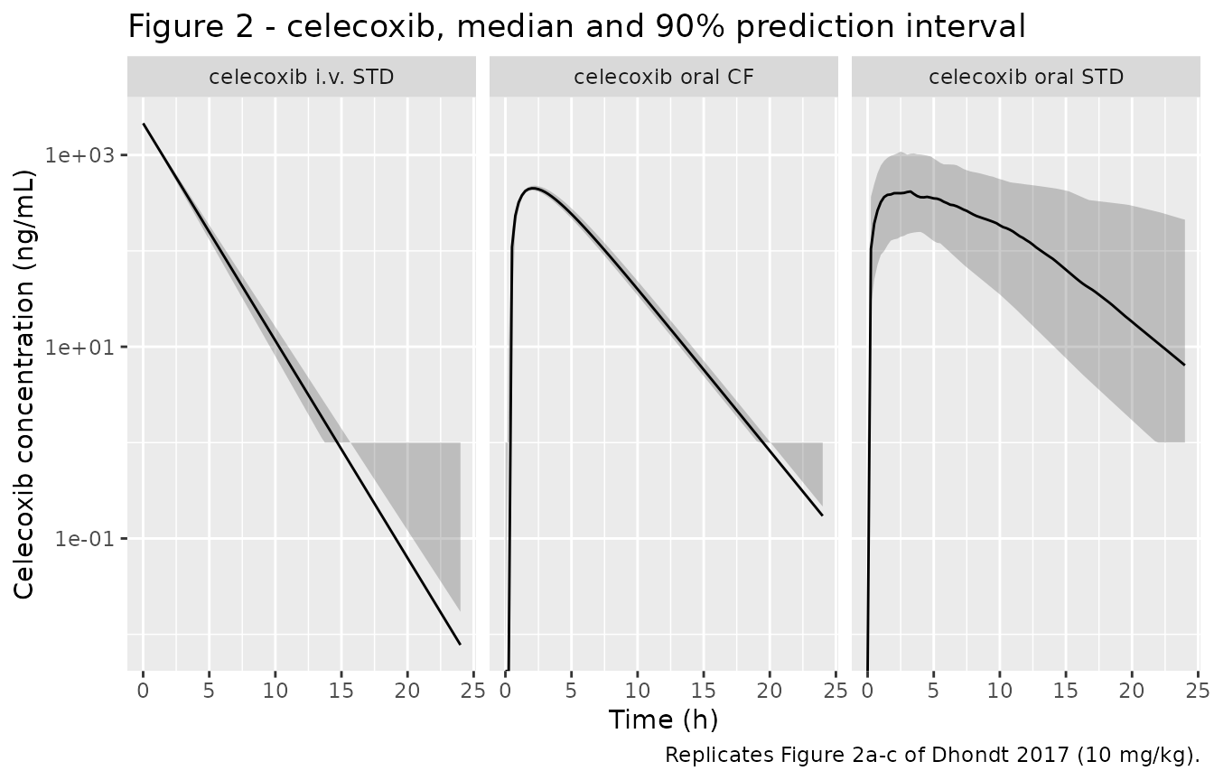
# Replicates Figure 3a-c of Dhondt 2017: mavacoxib after i.v. STD, oral STD
# and oral CF administration over the full 1008 h window.
ggplot(vpc_band("mavacoxib", 1008), aes(time, Q50)) +
  geom_ribbon(aes(ymin = pmax(Q05, 0.1), ymax = Q95), alpha = 0.25) +
  geom_line() +
  facet_wrap(~arm) +
  scale_y_log10() +
  labs(
    x = "Time (h)", y = "Mavacoxib concentration (ng/mL)",
    title = "Figure 3 - mavacoxib, median and 90% prediction interval",
    caption = "Replicates Figure 3a-c of Dhondt 2017 (4 mg/kg, 42-day window)."
  )
#> Warning in scale_y_log10(): log-10 transformation introduced infinite values.
#> log-10 transformation introduced infinite values.
#> log-10 transformation introduced infinite values.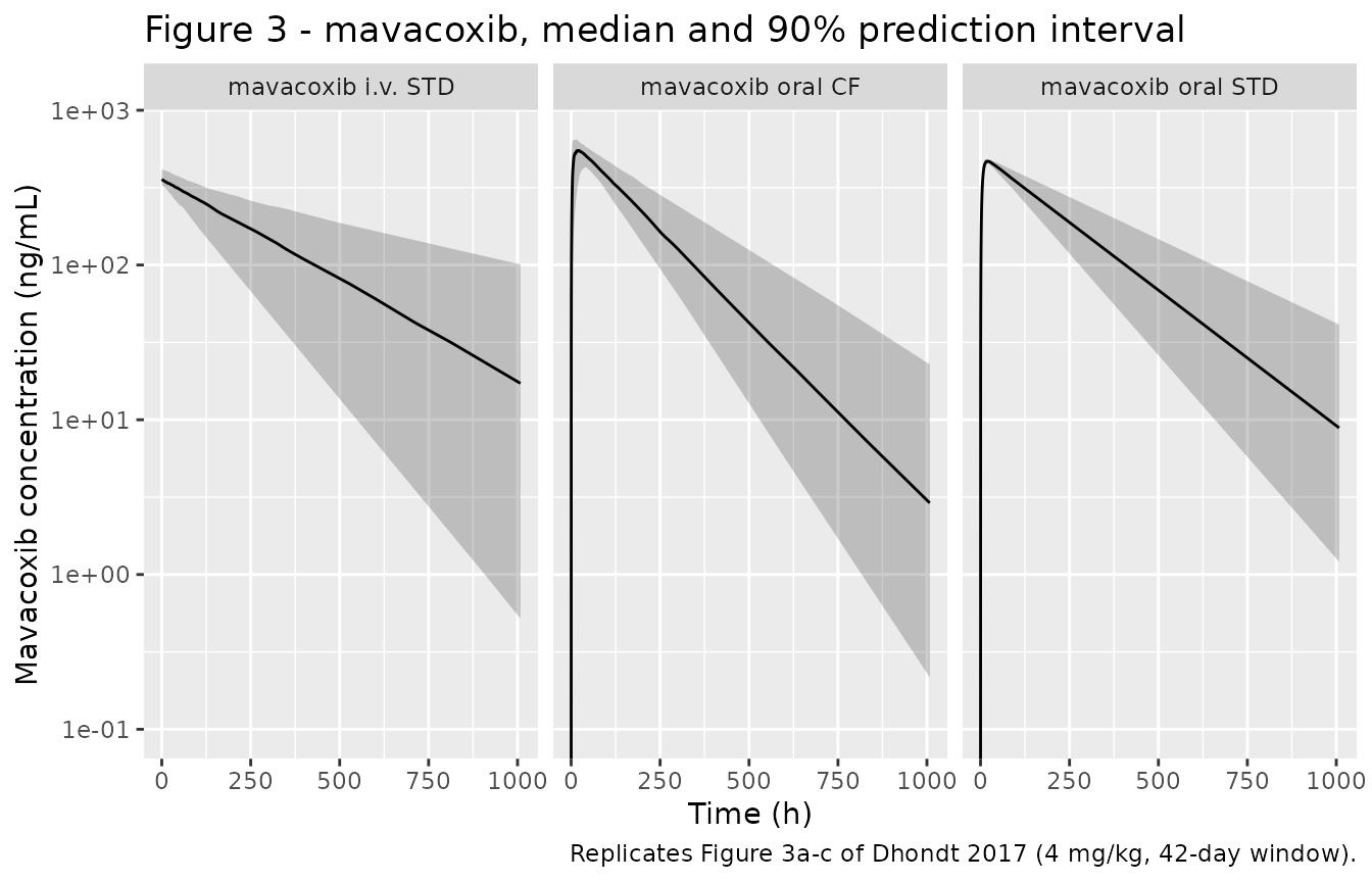
# Replicates Figure 4a-b of Dhondt 2017: meloxicam after i.v. and oral
# administration of the commercial formulation.
ggplot(vpc_band("meloxicam", 24), aes(time, Q50)) +
  geom_ribbon(aes(ymin = pmax(Q05, 0.01), ymax = Q95), alpha = 0.25) +
  geom_line() +
  facet_wrap(~arm, scales = "free_y") +
  scale_y_log10() +
  labs(
    x = "Time (h)", y = "Meloxicam concentration (ng/mL)",
    title = "Figure 4 - meloxicam, median and 90% prediction interval",
    caption = "Replicates Figure 4a-b of Dhondt 2017 (1 mg/kg)."
  )
#> Warning in scale_y_log10(): log-10 transformation introduced infinite values.
#> log-10 transformation introduced infinite values.
#> log-10 transformation introduced infinite values.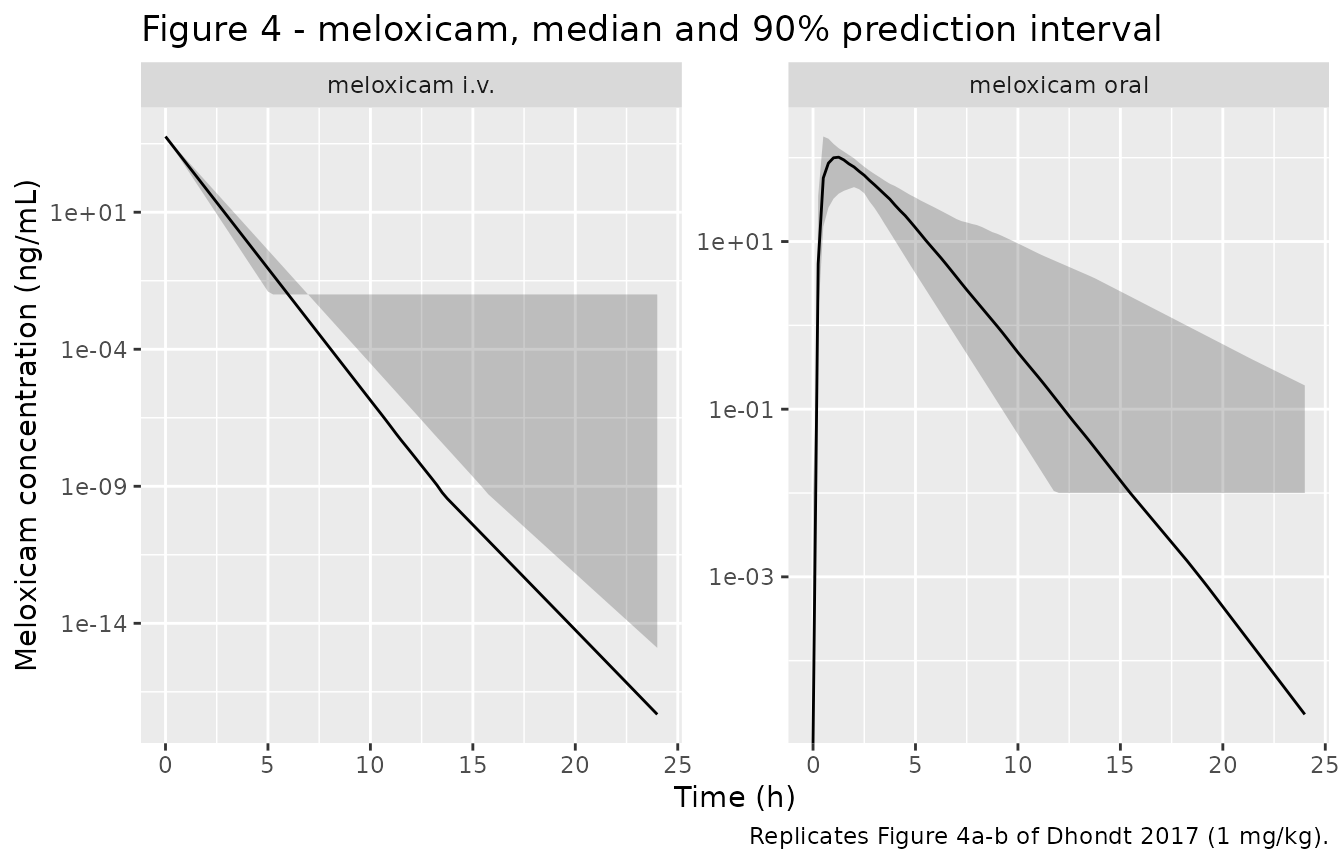
The qualitative contrast the paper draws is reproduced: celecoxib and meloxicam are essentially cleared within a day, whereas mavacoxib is still measurable at 1008 h. The meloxicam panels also show the low oral exposure behind the 11% bioavailability – an oral Cmax around 100 ng/mL against an intravenous C0 near 5800 ng/mL at the same 1 mg/kg dose.
The source’s meloxicam profiles show a secondary concentration rise 1-2 h after the intravenous dose and about 4 h after the oral dose, which the authors ascribe to enterohepatic recycling. The selected structural model has a single elimination pathway and no recycling, so the simulated curves are monotone after the peak; that is a property of the published model, not of the encoding.
PKNCA validation
The NCA is run on the noise-free typical-value profile of each arm.
That is the right comparator here because the paper’s Cmax,
Tmax, AUC0-inf and T1/2el are the
fitted model’s secondary parameters at the typical
values, not non-compartmental estimates from the raw observations.
nca_grid <- list(
  celecoxib = sort(unique(c(seq(0, 12, by = 0.02), seq(12, 24, by = 0.1)))),
  mavacoxib = sort(unique(c(seq(0, 48, by = 0.1), seq(48, 1008, by = 2)))),
  meloxicam = sort(unique(c(seq(0, 12, by = 0.02), seq(12, 24, by = 0.1))))
)

solve_typical <- function(i) {
  grid <- nca_grid[[arms$drug[i]]]
  ev <- dplyr::bind_rows(
    tibble::tibble(id = 1L, time = 0, amt = arms$dose[i], evid = 1L, cmt = arms$dose_cmt[i]),
    tibble::tibble(id = 1L, time = grid, amt = NA_real_, evid = 0L, cmt = "central")
  ) |>
    dplyr::arrange(time, dplyr::desc(evid))
  out <- rxode2::rxSolve(
    rxode2::zeroRe(mods[[arms$arm[i]]]),
    events = ev, omega = NA, useLinCmt = FALSE
  ) |>
    as.data.frame()
  tibble::tibble(id = 1L, time = out$time, Cc = out$Cc, arm = arms$arm[i])
}

tv <- dplyr::bind_rows(lapply(seq_len(nrow(arms)), solve_typical))
#> ℹ parameter labels from comments will be replaced by 'label()'
#> ℹ parameter labels from comments will be replaced by 'label()'
#> ℹ parameter labels from comments will be replaced by 'label()'
#> ℹ parameter labels from comments will be replaced by 'label()'
#> ℹ parameter labels from comments will be replaced by 'label()'
#> ℹ parameter labels from comments will be replaced by 'label()'
#> ℹ parameter labels from comments will be replaced by 'label()'
#> ℹ parameter labels from comments will be replaced by 'label()'

stopifnot(all(tv$Cc >= 0), !anyNA(tv$Cc))

# Use only `!is.na(Cc)` as the filter: dropping `time == 0` or `Cc == 0` rows
# would remove the anchor PKNCA needs for AUC0-*.
tv_conc <- tv |>
  dplyr::filter(!is.na(Cc)) |>
  dplyr::select(id, time, Cc, arm)

# Time-zero anchor. The oral arms are extravascular, so the pre-dose
# concentration is zero; the intravenous arms are boluses whose t = 0
# concentration is C0 = dose/Vd and is already on the grid.
tv_conc <- dplyr::bind_rows(
  tv_conc,
  tv_conc |>
    dplyr::distinct(id, arm) |>
    dplyr::mutate(time = 0, Cc = 0)
) |>
  dplyr::distinct(arm, id, time, .keep_all = TRUE) |>
  dplyr::arrange(arm, id, time)

stopifnot(all(
  tv_conc |>
    dplyr::group_by(arm) |>
    dplyr::summarise(has0 = any(time == 0), .groups = "drop") |>
    dplyr::pull(has0)
))

dose_df <- arms |>
  dplyr::transmute(
    id = 1L, time = 0, amt = dose, arm,
    route = ifelse(dose_cmt == "central", "intravascular", "extravascular")
  )

nca_res <- PKNCA::pk.nca(PKNCA::PKNCAdata(
  PKNCA::PKNCAconc(tv_conc, Cc ~ time | arm + id),
  PKNCA::PKNCAdose(dose_df, amt ~ time | arm + id, route = "route"),
  intervals = data.frame(
    start = 0, end = Inf,
    cmax = TRUE, tmax = TRUE, aucinf.obs = TRUE, half.life = TRUE
  )
))
Comparison against the published values
cmp <- nlmixr2lib::ncaComparisonTable(
  simulated = nca_res,
  reference = printed |> dplyr::select(-ke, -tmax),
  by = "arm",
  units = c(cmax = "ng/mL", aucinf.obs = "ng*h/mL", half.life = "h"),
  tolerance_pct = 20
)

knitr::kable(
  cmp,
  caption = paste(
    "PKNCA on the typical-value profile against the secondary parameters",
    "printed in Dhondt 2017 Tables 1-3. * differs from the reference by more",
    "than 20%."
  )
)| NCA parameter | arm | Reference | Simulated | % diff |
|---|---|---|---|---|
| Cmax (ng/mL) | celecoxib i.v. STD | 2140 | 2140 | -0.0% |
| Cmax (ng/mL) | celecoxib oral STD | 536 | 529 | -1.3% |
| Cmax (ng/mL) | celecoxib oral CF | 455 | 453 | -0.5% |
| Cmax (ng/mL) | mavacoxib i.v. STD | 364 | 364 | +0.1% |
| Cmax (ng/mL) | mavacoxib oral STD | 470 | 471 | +0.2% |
| Cmax (ng/mL) | mavacoxib oral CF | 585 | 584 | -0.1% |
| Cmax (ng/mL) | meloxicam i.v. | 5780 | 5780 | +0.1% |
| Cmax (ng/mL) | meloxicam oral | 102 | 102 | +0.1% |
| AUC0-∞ (obs) (ng*h/mL) | celecoxib i.v. STD | 4140 | 4130 | -0.2% |
| AUC0-∞ (obs) (ng*h/mL) | celecoxib oral STD | 4570 | 4570 | -0.1% |
| AUC0-∞ (obs) (ng*h/mL) | celecoxib oral CF | 2310 | 2310 | +0.1% |
| AUC0-∞ (obs) (ng*h/mL) | mavacoxib i.v. STD | 111000 | 111000 | -0.1% |
| AUC0-∞ (obs) (ng*h/mL) | mavacoxib oral STD | 126000 | 129000 | +2.3% |
| AUC0-∞ (obs) (ng*h/mL) | mavacoxib oral CF | 123000 | 121000 | -1.4% |
| AUC0-∞ (obs) (ng*h/mL) | meloxicam i.v. | 2580 | 2580 | +0.1% |
| AUC0-∞ (obs) (ng*h/mL) | meloxicam oral | 295 | 296 | +0.2% |
| t½ (h) | celecoxib i.v. STD | 1.34 | 1.34 | -0.2% |
| t½ (h) | celecoxib oral STD | 1.86 | 2.74 | +47.3%* |
| t½ (h) | celecoxib oral CF | 0.88 | 1.8 | +104.4%* |
| t½ (h) | mavacoxib i.v. STD | 212 | 212 | -0.2% |
| t½ (h) | mavacoxib oral STD | 172 | 176 | +2.3% |
| t½ (h) | mavacoxib oral CF | 135 | 133 | -1.5% |
| t½ (h) | meloxicam i.v. | 0.31 | 0.313 | +0.9% |
| t½ (h) | meloxicam oral | 0.9 | 0.912 | +1.3% |
Tmax is left out of this table because it is zero for
the four intravenous arms and a percentage difference against zero is
undefined; the Tmax rows were already checked in the
closed-form table above, where every arm agrees to better than 1%.
Cmax and AUC0-inf agree throughout.
Half-life is the one place where PKNCA and the paper
legitimately disagree, and only for the two celecoxib oral
arms. Both of those are flip-flop systems: Ka
(0.27 and 0.39 /h) is smaller than the apparent elimination rate
Ke (0.37 and 0.79 /h), so the observable terminal slope of
the curve is absorption-limited and reflects Ka, while the
T1/2el the paper prints is ln(2)/Ke, a
computed model quantity that is not observable in these profiles. PKNCA
is measuring the real terminal slope and is right to report a different
number; nothing is tuned to close the gap.
flip <- nca_res |>
  as.data.frame() |>
  dplyr::filter(PPTESTCD == "half.life") |>
  dplyr::select(arm, half.life = PPORRES) |>
  dplyr::left_join(
    tibble::tibble(
      arm = arms$arm,
      ka = vapply(arms$arm, function(a) {
        th <- uis[[a]]$theta
        if ("lka" %in% names(th)) exp(th[["lka"]]) else NA_real_
      }, numeric(1)),
      ke = vapply(arms$arm, function(a) {
        th <- uis[[a]]$theta
        exp(th[["lcl"]]) / exp(th[["lvc"]])
      }, numeric(1))
    ),
    by = "arm"
  ) |>
  dplyr::mutate(
    flip_flop = !is.na(ka) & ka < ke,
    `expected terminal rate` = ifelse(flip_flop, ka, ke),
    `expected t1/2 (h)` = log(2) / `expected terminal rate`,
    `% difference` = 100 * (half.life - `expected t1/2 (h)`) / `expected t1/2 (h)`,
    `t1/2 from Ka (h)` = log(2) / ka,
    `t1/2 from Ke (h)` = log(2) / ke
  )

flip |>
  dplyr::select(arm, ka, ke, flip_flop, `expected t1/2 (h)`,
                `PKNCA t1/2 (h)` = half.life, `% difference`) |>
  dplyr::rename("Arm" = arm, "Ka (1/h)" = ka, "Ke (1/h)" = ke,
                "Flip-flop?" = flip_flop) |>
  knitr::kable(digits = 4,
caption = "PKNCA half-life against the slower of Ka and Ke for each arm.")| Arm | Ka (1/h) | Ke (1/h) | Flip-flop? | expected t1/2 (h) | PKNCA t1/2 (h) | % difference |
|---|---|---|---|---|---|---|
| celecoxib i.v. STD | NA | 0.5182 | FALSE | 1.3376 | 1.3376 | 0.0000 |
| celecoxib oral CF | 0.39 | 0.7869 | TRUE | 1.7773 | 1.7989 | 1.2165 |
| celecoxib oral STD | 0.27 | 0.3731 | TRUE | 2.5672 | 2.7391 | 6.6964 |
| mavacoxib i.v. STD | NA | 0.0033 | FALSE | 211.6024 | 211.6024 | 0.0000 |
| mavacoxib oral CF | 0.28 | 0.0052 | FALSE | 133.3783 | 133.4398 | 0.0461 |
| mavacoxib oral STD | 0.20 | 0.0039 | FALSE | 175.5228 | 175.7015 | 0.1019 |
| meloxicam i.v. | NA | 2.2428 | FALSE | 0.3091 | 0.3129 | 1.2399 |
| meloxicam oral | 1.19 | 0.7682 | FALSE | 0.9023 | 0.9116 | 1.0280 |
# Gate 1: exactly two arms are flip-flop, and both are celecoxib oral arms.
stopifnot(sum(flip$flip_flop, na.rm = TRUE) == 2L)
stopifnot(all(grepl("^celecoxib oral", flip$arm[flip$flip_flop])))

# Gate 2: PKNCA's terminal half-life tracks ln(2) divided by the SLOWER of the
# two rate constants, which is the definition of the observable terminal phase.
# The non-flip-flop arms are clean mono-exponential tails and must agree to
# better than 1.5%. The celecoxib oral arms are looser because Ke/Ka is only
# 1.38 and 2.02 there, so the two exponentials separate slowly and the last
# sampled decade still carries a little curvature; 8% is the observed gap and
# nothing is tuned to close it.
stopifnot(all(abs(flip$`% difference`[!flip$flip_flop]) < 1.5))
stopifnot(all(abs(flip$`% difference`[flip$flip_flop]) < 8))

# Gate 3 -- the discriminating one. For the flip-flop arms the measured
# half-life must sit far closer to the absorption-limited value than to the
# paper's Ke-derived T1/2el. That is the claim being made, and it is what
# separates a flip-flop result from a mis-transcribed clearance or volume.
ff <- flip[flip$flip_flop, ]
stopifnot(all(
  abs(ff$half.life - ff$`t1/2 from Ka (h)`) <
    0.25 * abs(ff$half.life - ff$`t1/2 from Ke (h)`)
))
Absolute oral bioavailability
The paper derives F% as the ratio of the oral to the
intravenous AUC0-inf at equal doses (Methods equation (8)).
Because that ratio is a function of the two arms’ Cl
estimates alone, it can be recomputed from the packaged models and
checked against the reported percentages.
cl_of <- function(arm_label) {
  th <- uis[[arm_label]]$theta
  exp(th[["lcl"]])
}

f_tbl <- tibble::tribble(
  ~`Oral arm`,           ~`i.v. arm`,          ~`Reported F%`,
  "celecoxib oral STD",  "celecoxib i.v. STD",            110,
  "celecoxib oral CF",   "celecoxib i.v. STD",             56,
  "mavacoxib oral STD",  "mavacoxib i.v. STD",            113,
  "mavacoxib oral CF",   "mavacoxib i.v. STD",            111,
  "meloxicam oral",      "meloxicam i.v.",                 11
) |>
  dplyr::mutate(
    `Recomputed F%` = 100 * vapply(`i.v. arm`, cl_of, numeric(1)) /
      vapply(`Oral arm`, cl_of, numeric(1)),
    `Absolute difference (pp)` = `Recomputed F%` - `Reported F%`
  )

knitr::kable(f_tbl, digits = 1,
caption = "Absolute oral bioavailability recomputed as Cl(i.v.)/(Cl/F)(oral).")| Oral arm | i.v. arm | Reported F% | Recomputed F% | Absolute difference (pp) |
|---|---|---|---|---|
| celecoxib oral STD | celecoxib i.v. STD | 110 | 110.5 | 0.5 |
| celecoxib oral CF | celecoxib i.v. STD | 56 | 56.0 | 0.0 |
| mavacoxib oral STD | mavacoxib i.v. STD | 113 | 116.1 | 3.1 |
| mavacoxib oral CF | mavacoxib i.v. STD | 111 | 109.1 | -1.9 |
| meloxicam oral | meloxicam i.v. | 11 | 11.5 | 0.5 |
# Mavacoxib's Cl/F is printed to two significant figures, which is worth a few
# percentage points on this ratio; celecoxib and meloxicam are printed to three
# and must land within one point.
stopifnot(all(abs(f_tbl$`Absolute difference (pp)`) < 6))
stopifnot(
  all(abs(f_tbl$`Absolute difference (pp)`[
    grepl("^(celecoxib|meloxicam)", f_tbl$`Oral arm`)
  ]) < 1)
)
The recomputed percentages land on the reported ones, confirming that the clearance estimates carried into the eight files are the ones the paper’s bioavailability conclusions rest on: essentially complete absorption of mavacoxib from both formulations, complete absorption of the celecoxib standard solution but only 56% from the ground tablet, and a strikingly low 11% for the meloxicam oral suspension.
Assumptions and deviations
-
Scale of the
omegacolumn (load-bearing). Tables 1-3 head the interindividual-variability columnomegaand each caption glosses it as “variance of the interindividual variability”. That contradicts Methods equation (4), which defines the random effect as having varianceomega^2and then states “Interindividual variability is reported asomega”. The equations are taken as authoritative and the tabulated values are read as standard deviations, squared here because nlmixr2ini()omega entries are variances. Two things support that reading. First, the same captions callsigma_multandsigma_add“variances”, yet Methods equation- forms the ratio
sigma_mult / sigma_addand multiplies it by a concentration – an operation that is only dimensionally coherent if both are standard deviations, so “variance” is demonstrably loose terminology in this paper. Second, Phoenix NLME, the software used, parameterises residual error by standard deviation. Under the alternative (variance) reading every IIV would be inflated – for instance celecoxib’s intravenousClwould go from about 4% CV to about 21% CV – with no change to any typical value or to any gate in this vignette, all of which test the structural parameters.
- forms the ratio
-
omegavalues printed as “< 0.001” (celecoxib i.v.Vd, celecoxib oral CFVd/FandKa, meloxicam i.v.Vd, meloxicam oralVd/FandTlag) are encoded at the printed upper bound, i.e. a variance of1e-06. Encoding them as exactly zero would make the OMEGA matrix singular and breakrxSolve’s Cholesky sampler; the bound keeps the fitted structure visible while staying positive definite. At a CV of 0.1% these etas are numerically inert. -
Equation (7) is reproduced as
add() + prop(). The printed form,C_obs = C_pred + eps * sqrt(1 + C_pred^(2*(sigma_mult/sigma_add)^2)), raises a concentration to a dimensionless power and is not a usable error model. It is a typesetting error for Phoenix NLME’s mix-ratio model,C_obs = C_pred + eps * sqrt(1 + C_pred^2 * (sigma_mult/sigma_add)^2), whose residual standard deviation issqrt(sigma_add^2 + (sigma_mult * C_pred)^2)– exactly nlmixr2’s default combinedadd() + prop(). Under that reading the celecoxib oral CF block’s two residual rows fall into place:sigma_mult= 0.41 is the proportional term and the block’s remainingRes. Error= 15.18 is the additive term in ng/mL. It is the only arm in the paper with two residual rows, which is what a two-parameter error model requires. -
The enterohepatic-recycling variant of the meloxicam model
is not packaged. Table 3 reports an intravenous meloxicam fit
that adds enterohepatic recycling (“IV CF 2”), but Table 4 rejects it –
AIC 542.13 and BIC 560.45 against 531.72 and 539.36 without recycling –
and the Results text states the recycling did not improve the fit. Per
the standing policy, rejected structural alternatives are not carried.
Two further reasons apply here: the paper does not write out the
recycling equations (it cites Gabrielsson and Weiner, which was not
available), and that block’s own printed secondary parameters are
internally inconsistent, giving
C0= 385.515 ng/mL andAUC0-inf= 149.05 ng.h/mL where itsVd= 0.148 L/kg andCl= 0.383 L/h/kg imply 6757 ng/mL and 2611 ng.h/mL. No oral meloxicam recycling fit is reported at all. -
No bioavailability parameter is encoded in the oral
models. The paper reports
Vd/FandCl/Fand computesF%afterwards from the AUC ratio, so the full dose enters the depot andFis absorbed into the apparent parameters. This is the authors’ own parameterisation; adding an explicitf(depot)would double-count it. -
Body weight and sex are documented but unused. Both
were screened by stepwise forward-backward selection and neither reached
the p < 0.01 inclusion threshold for any drug, so they appear in each
model’s
covariatesDataExcludedmetadata rather than incovariateData. The paper does not state which sex was the reference category, which is moot since the effect was not retained. - Virtual cohorts. The observed data are available from the corresponding author on request and are not published in machine-readable form, so the figures use 100 simulated birds per arm rather than the paper’s 22-40. Body weight is not a model covariate, so no covariate distribution had to be assumed.
- Typographic errors in the source, noted but not consequential. The Methods section “Mavacoxib PK study” states that “IV and PO dosing of celecoxib STD was performed … to 40 cockatiels” inside the mavacoxib experiment; from the surrounding text, Table 2 and the study design this is plainly mavacoxib. The abstract gives mavacoxib’s oral half-life as 135 h and the Results give the intravenous value as 212 h; both match their respective table rows and are consistent.
-
No erratum applies. A EuropePMC
commentCorrectionListquery for PMC5612971 returns nothing, and the article’s supplementary material contains only the LC-MS/MS validation tables (S1, S2) and goodness-of-fit and Q-Q plots (S1-S3) – no additional model parameters.