Lumiracoxib in rats (Vasquez-Bahena 2009)
Source:vignettes/articles/VasquezBahena_2009_lumiracoxib_rat.Rmd
VasquezBahena_2009_lumiracoxib_rat.RmdModel and source
- Citation: Vasquez-Bahena DA, Salazar-Morales UE, Ortiz MI, Castaneda-Hernandez G, Troconiz IF. Pharmacokinetic-pharmacodynamic modelling of the analgesic effects of lumiracoxib, a selective inhibitor of cyclooxygenase-2, in rats. Br J Pharmacol. 2010;159(1):176-187. doi:10.1111/j.1476-5381.2009.00508.x
- Description: Preclinical (rat). Two-compartment population PK plus indirect-response PK/PD model for the antinociceptive effect of oral lumiracoxib in carrageenan-induced thermal hyperalgesia in female Wistar rats (Vasquez-Bahena 2009). PK: first-order absorption with lag time and dose-dependent relative bioavailability. PD: time-variant (gamma function) carrageenan-induced COX-2 synthesis with first-order COX-2 degradation; lumiracoxib reversibly inactivates COX-2 via a competitive binding model (COX-2_act = KD * COX-2 / (KD + Cp)). The level of inflammatory mediators (MED) equals the active COX-2 amount and drives the paw withdrawal latency response LT = LT0 / (1 + MED).
- Article: https://doi.org/10.1111/j.1476-5381.2009.00508.x
Population
Two combined experiments in female Wistar rats (180-200 g, fasted overnight, free access to water; Methods, Animals). Experiment I (60 rats, six groups of 10) tested 1, 3, 10 and 30 mg/kg oral lumiracoxib co-administered with a 1 % carrageenan intraplantar injection in the right hind paw, plus a saline-injected group and a carrageenan-only group. Experiment II (20 rats, three groups) delivered 10 or 30 mg/kg oral lumiracoxib 4 hours after the carrageenan injection, plus a carrageenan + vehicle control. PK samples were drawn from the caudal artery at 13 nominal time points covering 5 min to 10 h after dosing in experiment I only; the paw-withdrawal latency response was measured in both experiments via the Hargreaves thermal plantar test (cut-off 30 s) at 9 time points in experiment I (1-10 h) and 16 time points in experiment II (1-24 h).
The same information is available programmatically via the model’s
population metadata
(rxode2::rxode2(readModelDb("VasquezBahena_2009_lumiracoxib_rat"))$population).
Source trace
The per-parameter origin is recorded as an in-file comment next to
each ini() entry in
inst/modeldb/specificDrugs/VasquezBahena_2009_lumiracoxib_rat.R.
The table below collects them in one place for review.
| Equation / parameter | Value | Source location |
|---|---|---|
ka |
15.2 1/h | Table 1 (p. 181) |
cl |
0.16 L/h | Table 1 |
vc |
0.49 L | Table 1 |
q |
0.42 L/h | Table 1 |
vp (VT) |
0.99 L | Table 1 |
tlag |
0.06 h | Table 1 |
imax_frel |
0.67 | Table 1 |
d50_frel |
4.3 mg/kg | Table 1 |
lfrel IIV anchor |
fixed at log(1) | Table 1 IIV row |
ks_cox2_saline (saline-only) |
0.21 COX-2/h | Table 3 footnote a (p. 183) |
a_cox2 (gamma amplitude) |
1.42 | Table 3 ‘Experiment I and II’ |
alpha_cox2 (gamma shape) |
1.3 | Table 3 |
beta_cox2 (gamma decay) |
0.33 1/h | Table 3 |
kd_cox2 (COX-2 degradation) |
0.89 1/h | Table 3 |
kd_drug (KD) |
0.24 ug/mL | Table 3 |
lt0 (baseline latency) |
14.3 s | Table 3 |
addSd (PK additive) |
0.037 ug/mL | Table 1 |
propSd (PK proportional) |
22 % | Table 1 |
addSd_LT (PD additive) |
2.4 s | Table 3 |
| IIV CV%: CL, Vc, ka | 36, 39, 92 % | Table 1 |
| IIV CV%: Frel | 18 % | Table 1 |
| IIV CV%: KD, LT0 | 62, 13 % | Table 3 |
| Eq. 1: LT = LT0/(1 + MED) | n/a | p. 179, Eq. 1 |
| Eq. 2: dCOX-2/dt | n/a | p. 179, Eq. 2 |
| Eq. 3: ks_COX-2(t) = A * t^alpha * exp(-beta * t) | n/a | p. 179, Eq. 3 |
| Eq. 4: COX-2_act competitive binding | n/a | p. 179, Eq. 4 |
| Frel = 1 - IMAX * D / (D + D50) | n/a | Table 1 formula row |
Virtual cohort
The original observed data are not publicly available. The cohort below mimics the published dose schedule for experiment I (six groups of 10 rats; doses 0, 0, 1, 3, 10, 30 mg/kg orally administered concurrently with intraplantar carrageenan or saline at t = 0). Body weights are drawn uniformly across the reported 180-200 g range.
set.seed(20260516L)

n_per_group <- 10L
groups <- tibble::tribble(
  ~group, ~treatment,            ~dose_mgkg, ~carrageenan,
  "I",    "Saline",                 0,        0L,
  "II",   "Carrageenan only",        0,        1L,
  "III",  "Carrageenan + 1 mg/kg",   1,        1L,
  "IV",   "Carrageenan + 3 mg/kg",   3,        1L,
  "V",    "Carrageenan + 10 mg/kg", 10,        1L,
  "VI",   "Carrageenan + 30 mg/kg", 30,        1L
)

make_cohort <- function(group_row, n, id_offset) {
  obs_times <- sort(unique(c(seq(0, 10, by = 0.1), seq(10, 24, by = 0.5))))
  ids <- id_offset + seq_len(n)
  wt  <- runif(n, 0.18, 0.20)
  ev_rows <- lapply(seq_len(n), function(j) {
    amt <- group_row$dose_mgkg * wt[j]
    dose_row <- data.frame(
      id = ids[j], time = 0, amt = amt, evid = 1L, cmt = 1L,
      dvid = NA_integer_,
      DOSE = group_row$dose_mgkg,
      CARRAGEENAN = group_row$carrageenan,
      WT = wt[j], treatment = group_row$treatment
    )
    obs_pk <- data.frame(
      id = ids[j], time = obs_times, amt = 0, evid = 0L, cmt = 0L,
      dvid = 1L,
      DOSE = group_row$dose_mgkg,
      CARRAGEENAN = group_row$carrageenan,
      WT = wt[j], treatment = group_row$treatment
    )
    obs_pd <- data.frame(
      id = ids[j], time = obs_times, amt = 0, evid = 0L, cmt = 0L,
      dvid = 2L,
      DOSE = group_row$dose_mgkg,
      CARRAGEENAN = group_row$carrageenan,
      WT = wt[j], treatment = group_row$treatment
    )
    # If dose is zero we still want PD observations but skip the empty dose.
    if (amt == 0) {
      dplyr::bind_rows(obs_pk, obs_pd)
    } else {
      dplyr::bind_rows(dose_row, obs_pk, obs_pd)
    }
  })
  dplyr::bind_rows(ev_rows)
}

events <- dplyr::bind_rows(
  Map(make_cohort,
      group_row = split(groups, seq_len(nrow(groups))),
      n         = rep(n_per_group, nrow(groups)),
      id_offset = (seq_len(nrow(groups)) - 1L) * n_per_group)
)
events <- events[order(events$id, events$time, -events$evid), ]
stopifnot(!anyDuplicated(unique(events[, c("id", "time", "evid", "dvid")])))
nrow(events)
#> [1] 15520
Simulation
mod <- rxode2::rxode2(readModelDb("VasquezBahena_2009_lumiracoxib_rat"))
#> ℹ parameter labels from comments will be replaced by 'label()'

# Typical-value replication (no IIV / no residual error) -- reproduces the
# population-typical trajectories shown in Figure 6 of the paper.
mod_typ <- rxode2::zeroRe(mod)
sim_typ <- rxode2::rxSolve(mod_typ, events, returnType = "data.frame",
                            keep = c("DOSE", "CARRAGEENAN", "WT", "treatment"))
#> ℹ omega/sigma items treated as zero: 'etalcl', 'etalvc', 'etalka', 'etalfrel', 'etalkd_drug', 'etallt0'
#> Warning: multi-subject simulation without without 'omega'

# Stochastic replication (population IIV + residual error) -- reproduces
# the dispersion shown in Figure 4 of the paper.
sim_stoch <- rxode2::rxSolve(mod, events, returnType = "data.frame",
                              keep = c("DOSE", "CARRAGEENAN", "WT", "treatment"))
Replicate published figures
Figure 6, left panel: typical COX-2 time course after saline vs carrageenan
fig6_left <- sim_typ |>
  dplyr::filter(time <= 10, id %in% c(1L, 11L)) |>  # first rat of each control group
  dplyr::mutate(group = ifelse(CARRAGEENAN == 1L,
                                "Carrageenan", "Saline"))

ggplot(fig6_left, aes(time, cox2, linetype = group)) +
  geom_line(linewidth = 1) +
  scale_linetype_manual(values = c("Saline" = "dashed", "Carrageenan" = "solid")) +
  labs(x = "Time (h)", y = "COX-2 (arbitrary units)",
       linetype = NULL,
       title = "Figure 6 left -- Typical COX-2 time course",
       caption = "Replicates Figure 6 left panel of Vasquez-Bahena 2009.")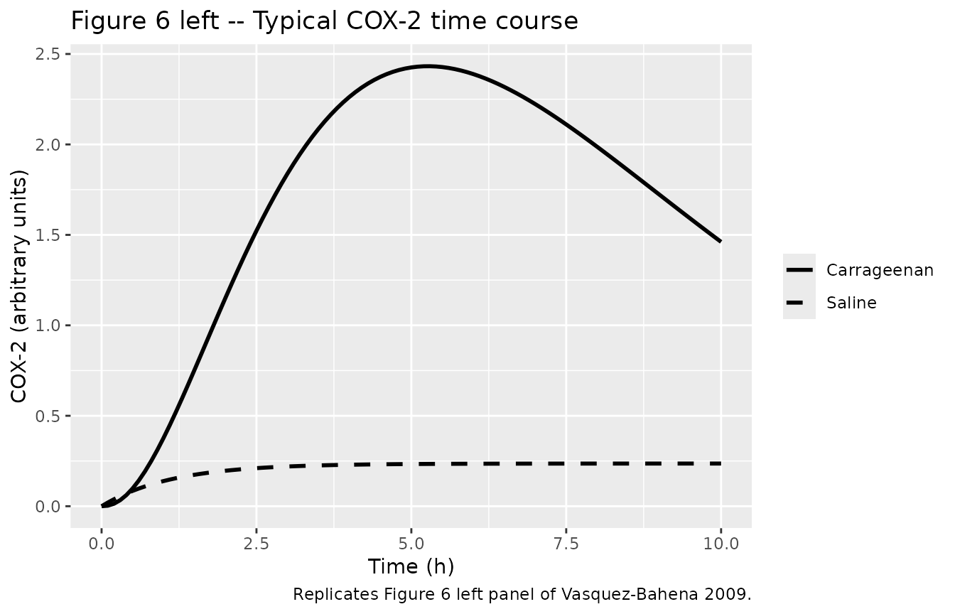
Figure 6, right panel: COX-2_act vs lumiracoxib plasma concentration
cp_grid <- seq(0, 5, length.out = 200)
fig6_right <- data.frame(
  Cp = cp_grid,
  COX2_act = 0.24 * 1 / (0.24 + cp_grid)
)

ggplot(fig6_right, aes(Cp, COX2_act)) +
  geom_line(linewidth = 1) +
  geom_vline(xintercept = 0.24, linetype = "dashed", colour = "gray40") +
  geom_hline(yintercept = 0.5, linetype = "dashed", colour = "gray40") +
  labs(x = "Plasma concentration (ug/mL)",
       y = "Fraction of active COX-2 (COX-2_act / COX-2)",
       title = "Figure 6 right -- COX-2 activity vs lumiracoxib Cp at KD = 0.24",
       caption = "Replicates Figure 6 right panel of Vasquez-Bahena 2009.")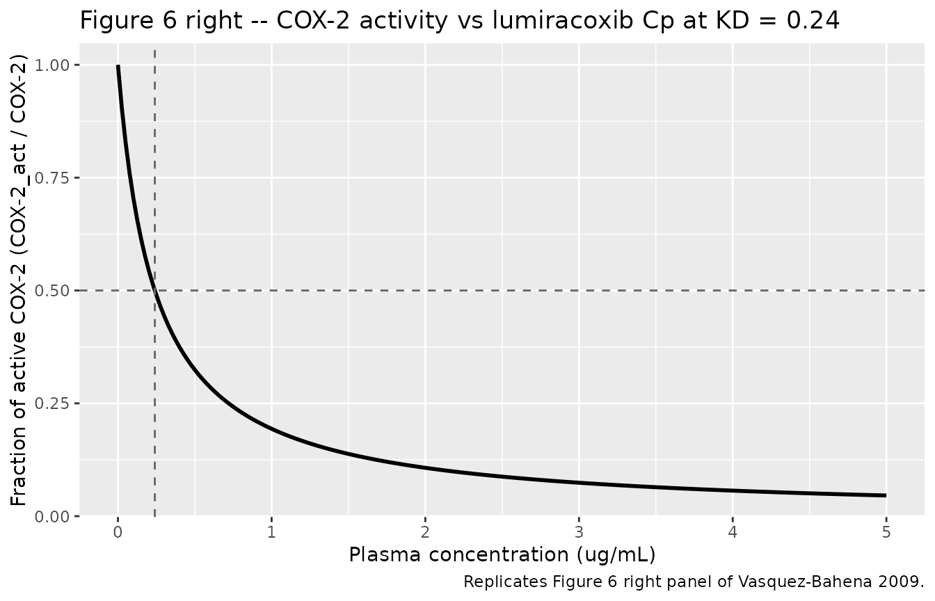
Figure 2A: typical plasma concentration profiles by dose
fig2A <- sim_typ |>
  dplyr::filter(DOSE > 0, time <= 10) |>
  dplyr::group_by(time, DOSE, treatment) |>
  dplyr::summarise(Cc_median = median(Cc, na.rm = TRUE), .groups = "drop") |>
  dplyr::mutate(dose_lab = factor(paste0(DOSE, " mg/kg"),
                                   levels = c("1 mg/kg","3 mg/kg",
                                              "10 mg/kg","30 mg/kg")))

ggplot(fig2A, aes(time, Cc_median, colour = dose_lab)) +
  geom_line(linewidth = 0.8) +
  scale_y_continuous(limits = c(0, NA)) +
  labs(x = "Time (h)", y = "Lumiracoxib plasma concentration (ug/mL)",
       colour = NULL,
       title = "Figure 2A -- Typical plasma profiles by oral dose",
       caption = "Replicates Figure 2 panel A of Vasquez-Bahena 2009.")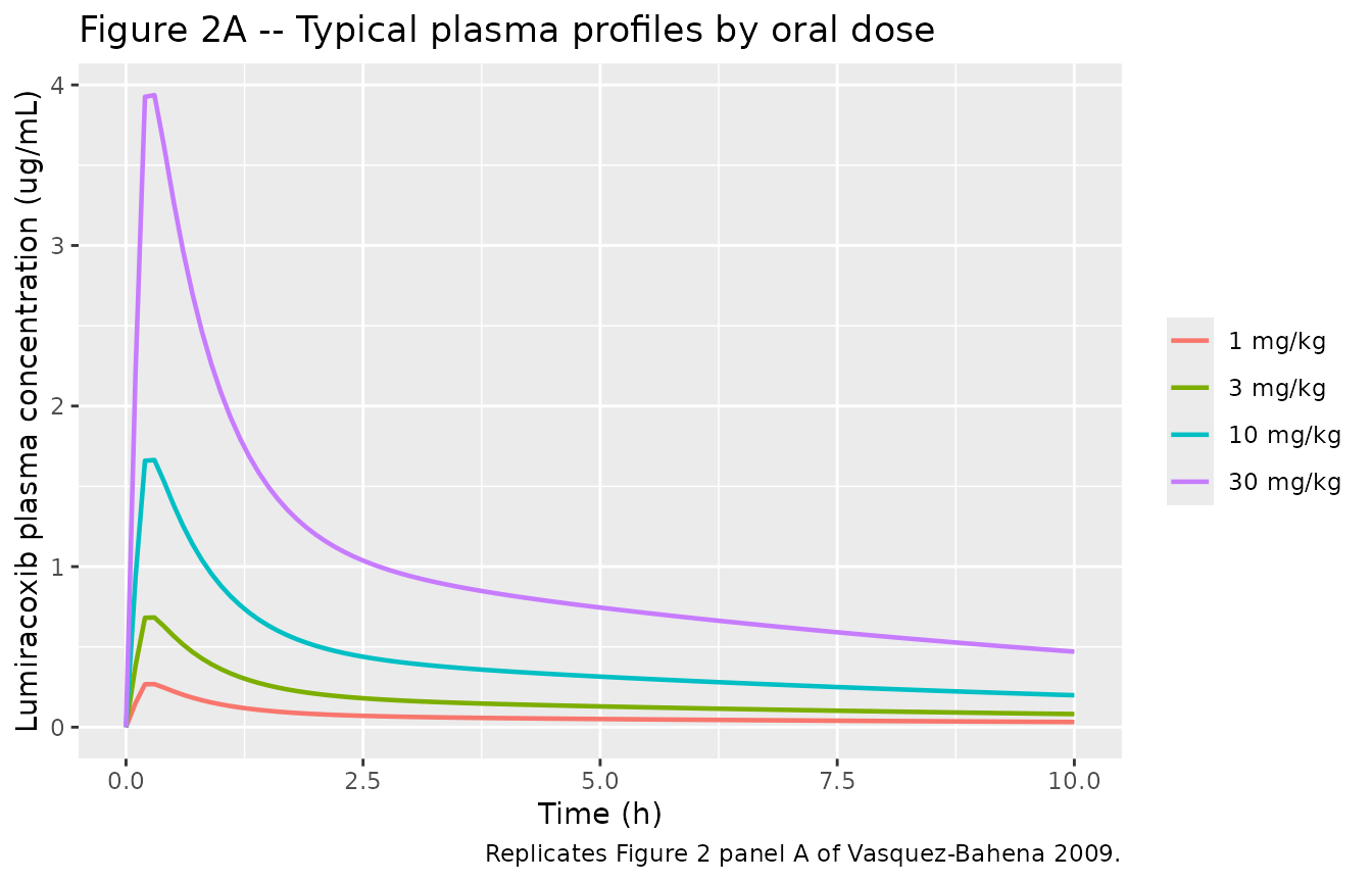
Figure 5: typical latency response trajectories by dose
fig5 <- sim_typ |>
  dplyr::filter(time <= 10) |>
  dplyr::group_by(time, treatment) |>
  dplyr::summarise(LT_median = median(LT, na.rm = TRUE), .groups = "drop")

ggplot(fig5, aes(time, LT_median, colour = treatment)) +
  geom_line(linewidth = 0.8) +
  labs(x = "Time (h)", y = "Latency time (s)",
       colour = NULL,
       title = "Figure 5 -- Typical latency response by dose group",
       caption = "Replicates Figure 5 of Vasquez-Bahena 2009 (experiment I).")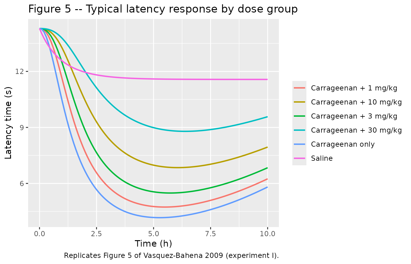
PKNCA validation (experiment I dose groups)
sim_pk <- sim_typ |>
  dplyr::filter(DOSE > 0, time <= 10) |>
  dplyr::distinct(id, time, DOSE, treatment, Cc) |>
  dplyr::filter(!is.na(Cc))

conc_obj <- PKNCA::PKNCAconc(sim_pk, Cc ~ time | treatment + id)

dose_df <- events |>
  dplyr::filter(evid == 1L, DOSE > 0) |>
  dplyr::distinct(id, time, amt, treatment, DOSE)

dose_obj <- PKNCA::PKNCAdose(dose_df, amt ~ time | treatment + id)

intervals <- data.frame(
  start = 0,
  end = 10,
  cmax = TRUE,
  tmax = TRUE,
  auclast = TRUE,
  half.life = TRUE
)

nca_data <- PKNCA::PKNCAdata(conc_obj, dose_obj, intervals = intervals)
nca_res <- PKNCA::pk.nca(nca_data)
nca_summary <- summary(nca_res)
knitr::kable(
  nca_summary,
  caption = "Simulated NCA parameters by dose group (typical-value rxSolve)."
)| start | end | treatment | N | auclast | cmax | tmax | half.life |
|---|---|---|---|---|---|---|---|
| 0 | 10 | Carrageenan + 1 mg/kg | 10 | 0.687 [2.87] | 0.268 [2.87] | 0.300 [0.300, 0.300] | 7.51 [3.35e-10] |
| 0 | 10 | Carrageenan + 10 mg/kg | 10 | 4.20 [3.37] | 1.64 [3.37] | 0.300 [0.300, 0.300] | 7.51 [0.00000103] |
| 0 | 10 | Carrageenan + 3 mg/kg | 10 | 1.73 [3.11] | 0.675 [3.11] | 0.300 [0.300, 0.300] | 7.51 [0.00000329] |
| 0 | 10 | Carrageenan + 30 mg/kg | 10 | 9.95 [3.26] | 3.89 [3.26] | 0.300 [0.300, 0.300] | 7.51 [6.73e-7] |
Comparison against published NCA
Table 2 of Vasquez-Bahena 2009 reports observed and 1000-replicate simulated Cmax and AUC0-last. The table below pairs the published values with the typical-value rxSolve summary above for orientation only – the published values are 1000-replicate stochastic means, while the rxSolve summary is the median of a 60-subject typical-value cohort.
paper_tab2 <- tibble::tribble(
  ~treatment,                ~paper_Cmax_obs, ~paper_Cmax_sim, ~paper_AUC0last_obs, ~paper_AUC0last_sim,
  "Carrageenan + 1 mg/kg",     0.33,            0.31,            0.20,                  0.18,
  "Carrageenan + 3 mg/kg",     0.94,            0.68,            1.23,                  0.94,
  "Carrageenan + 10 mg/kg",    1.45,            1.65,            3.63,                  3.70,
  "Carrageenan + 30 mg/kg",    3.64,            3.94,            9.40,                  8.70
)

sim_summary <- sim_typ |>
  dplyr::filter(DOSE > 0, time <= 10) |>
  dplyr::group_by(treatment, id) |>
  dplyr::summarise(
    Cmax = max(Cc, na.rm = TRUE),
    AUC0_10 = sum(diff(time) * (Cc[-1] + Cc[-length(Cc)]) / 2),
    .groups = "drop"
  ) |>
  dplyr::group_by(treatment) |>
  dplyr::summarise(
    Cmax_median   = median(Cmax),
    AUC0_10_median = median(AUC0_10),
    .groups = "drop"
  )

knitr::kable(
  dplyr::left_join(paper_tab2, sim_summary, by = "treatment"),
  caption = paste(
    "Side-by-side: paper Table 2 (observed and 1000-replicate simulated",
    "mean Cmax and AUC0-last) vs the typical-value rxSolve summary in this",
    "vignette. AUC values diverge at the lowest doses because Vasquez-",
    "Bahena 2009 reports AUC0-last truncated at the analytical LLOQ of",
    "0.10 ug/mL, while the rxSolve trapezoidal AUC integrates the full",
    "0-10 h window (which extends well below LLOQ at 1-3 mg/kg)."
  )
)| treatment | paper_Cmax_obs | paper_Cmax_sim | paper_AUC0last_obs | paper_AUC0last_sim | Cmax_median | AUC0_10_median |
|---|---|---|---|---|---|---|
| Carrageenan + 1 mg/kg | 0.33 | 0.31 | 0.20 | 0.18 | 0.2679583 | 0.6860838 |
| Carrageenan + 3 mg/kg | 0.94 | 0.68 | 1.23 | 0.94 | 0.6831060 | 1.7490337 |
| Carrageenan + 10 mg/kg | 1.45 | 1.65 | 3.63 | 3.70 | 1.6637535 | 4.2598957 |
| Carrageenan + 30 mg/kg | 3.64 | 3.94 | 9.40 | 8.70 | 3.9364377 | 10.0789052 |
PD comparison: latency-response minimums
Table 4 of Vasquez-Bahena 2009 reports the observed and
1000-replicate simulated mean minimum latency response
(LTmin) per group. The table below pairs the published
values with typical-value LT_min from the rxSolve
trajectories in this vignette for orientation only. The rxSolve typical
trajectory is uniformly higher than the paper’s reported simulated mean
because the paper’s simulated LTmin is the
across-time-point minimum of stochastic trajectories (additive residual
error SD 2.4 s pulls the minimum across nine to sixteen observation time
points down by several seconds relative to the smooth typical-value
curve). The qualitative ordering of LT_min across
treatments is reproduced.
paper_tab4 <- tibble::tribble(
  ~treatment,                ~paper_LTmin_obs, ~paper_LTmin_sim,
  "Saline",                       8.1,            8.3,
  "Carrageenan only",             1.9,            1.6,
  "Carrageenan + 1 mg/kg",        3.3,            2.3,
  "Carrageenan + 3 mg/kg",        3.9,            3.05,
  "Carrageenan + 10 mg/kg",       5.3,            4.4,
  "Carrageenan + 30 mg/kg",       6.5,            6.0
)

sim_lt <- sim_typ |>
  dplyr::group_by(treatment, id) |>
  dplyr::summarise(LT_min = min(LT, na.rm = TRUE), .groups = "drop") |>
  dplyr::group_by(treatment) |>
  dplyr::summarise(LT_min_median = median(LT_min), .groups = "drop")

knitr::kable(
  dplyr::left_join(paper_tab4, sim_lt, by = "treatment"),
  caption = paste(
    "Side-by-side: paper Table 4 (observed and 1000-replicate simulated mean",
    "LTmin) vs the typical-value rxSolve LT_min in this vignette. The",
    "typical-value column omits residual error (SD 2.4 s additive on LT)."
  )
)| treatment | paper_LTmin_obs | paper_LTmin_sim | LT_min_median |
|---|---|---|---|
| Saline | 8.1 | 8.30 | 11.570000 |
| Carrageenan only | 1.9 | 1.60 | 4.166283 |
| Carrageenan + 1 mg/kg | 3.3 | 2.30 | 4.734326 |
| Carrageenan + 3 mg/kg | 3.9 | 3.05 | 5.486400 |
| Carrageenan + 10 mg/kg | 5.3 | 4.40 | 6.846762 |
| Carrageenan + 30 mg/kg | 6.5 | 6.00 | 8.790065 |
Assumptions and deviations
Custom COX-2 state. The model uses a paper-specific state variable
cox2for the unobserved active COX-2 pool driving inflammatory mediators.cox2is not a registered canonical compartment inR/conventions.R::registeredCompartments;checkModelConventions()flags this with a warning. The name is kept paper-faithful because Vasquez-Bahena 2009 explicitly parameterises COX-2 turnover as the PD state (Methods, COX-2 model, Eq. 2-4) and reports parameters specifically for COX-2 synthesis and degradation.Frel encoding – IIV anchor. The paper estimates the dose-dependent relative bioavailability as
Frel = 1 - IMAX * D / (D50 + D)with exponential IIV on the whole formula (Table 1 IIV row, 18 %). To satisfy the nlmixr2lib convention that every IIVetalfrelpair with a fixed-effect parameterlfrel, anlfrel <- fixed(log(1))anchor is introduced and the dose-dependent reduction is applied as a multiplicative derived factor:frel = exp(lfrel + etalfrel) * (1 - imax_frel * DOSE / (d50_frel + DOSE)). This is mathematically equivalent to the paper’s specification and is the same pattern asIde_2009_pravastatin.Rin this package.DOSE units. The canonical
DOSEcovariate ininst/references/covariate-columns.mdis documented in mg; this model overrides per-covariateData[[DOSE]]$unitsto mg/kg because the source paper’sD50 = 4.3estimate is on the mg/kg scale (Table 1). When constructing the event table, supply DOSE in mg/kg as a per-subject covariate and supply the actual mg dose at the dose event asamt = DOSE * WT_kg(Methods, Study design).CARRAGEENAN covariate. Added as a new canonical entry in
inst/references/covariate-columns.mdalongside this extraction. CARRAGEENAN = 1 selects the gamma-function synthesis rateks_cox2(t) = A * t^alpha * exp(-beta * t)(Eq. 3); CARRAGEENAN = 0 selects the constant saline rateks_cox2_saline(Table 3 footnote a). Both scenarios start atcox2(0) = 0per the explicit assumption in Methods, COX-2 model, paragraph 2.LLOQ truncation. The paper reports
AUC0-lasttruncated at the analytical LLOQ of 0.10 ug/mL (Methods, Analysis of lumiracoxib in plasma). The rxSolve trapezoidal AUC in this vignette integrates the full 0-10 h window without truncation, so the simulated AUC for the 1 and 3 mg/kg groups is materially higher than the paper’s reported AUC0-last value. Cmax is unaffected because the peak always lies above LLOQ.Typical-value vs simulated-mean. This vignette reports the median of the typical-value (
zeroRe) trajectories. The paper’s predictive-check tables (Table 2, Table 4) report the mean of 1000 stochastic replicates with full IIV and residual error. The two will not match exactly; in particular the paper’s stochasticLTminis materially lower than the smooth typical-value trajectory’s minimum because the additive residual error (SD 2.4 s) propagates into the across-time-point minimum.