Evinacumab (Bihorel 2025)
Source:vignettes/articles/Bihorel_2025_evinacumab.Rmd
Bihorel_2025_evinacumab.Rmd
ui  <- rxode2::rxode(readModelDb("Bihorel_2025_evinacumab"))
#> ℹ parameter labels from comments will be replaced by 'label()'
mod <- rxode2::zeroRe(ui)   # typical-value engine: IIV and residual error switched off
Model and source
- Citation: Bihorel S, Dingman R, Mendell J, Wang Y, Banerjee P, Pordy R, Davis JD, DiCioccio AT, Harnisch L. Population pharmacokinetics and exposure-response modeling for evinacumab in children, adolescents, and adults with homozygous familial hypercholesterolemia. CPT Pharmacometrics Syst Pharmacol. 2025;14(11):1823-1834. doi:10.1002/psp4.70016. Refines the earlier model of Pu X et al. CPT Pharmacometrics Syst Pharmacol. 2021;10(11):1412-1421 (doi:10.1002/psp4.12711); see modellib(‘Pu_2021_evinacumab’).
- Description: Population PK/PD model for evinacumab in children (5 to <12 years), adolescents, and adults with homozygous familial hypercholesterolemia and in phase 1 participants (Bihorel 2025): two-compartment PK with first-order SC absorption (lag time, partial bioavailability) and parallel linear plus Michaelis-Menten elimination, with linear disposition parameters allometrically scaled by time-varying body weight, linked to a type 1 indirect-response model in which evinacumab inhibits LDL-C production and a second, time-varying LDL-C elimination process quantifies the lipoprotein-apheresis effect.
- Article: https://doi.org/10.1002/psp4.70016
- Supplement (final NONMEM control streams, Code 1 and Code 2): https://doi.org/10.1002/psp4.70016
This model refines the earlier evinacumab model of Pu 2021, which is
packaged separately as modellib("Pu_2021_evinacumab"). The
two are not interchangeable: this refinement
re-parameterises the disposition from first-order rate constants to
allometrically scaled clearances and volumes on
time-varying weight, extends the population down to age
5 years, estimates the LDL-C baseline instead of reading it from the
data, drops the race effect on Imax, and adds a
lipoprotein-apheresis elimination arm for LDL-C.
Every structural equation and every parameter value below was transcribed from the paper’s Tables 2 and 3 and from the two final NONMEM control streams printed in the Supporting Information, which fix several details the main text leaves implicit (see Source trace).
Population
The pooled population PK analysis used 322 participants from seven clinical studies: 183 phase 1 participants with elevated triglycerides and/or LDL-C but otherwise healthy, and 139 patients with homozygous familial hypercholesterolemia (HoFH). Age spanned 5 to 75 years (20 children aged 5 to <12 years, 14 adolescents aged 12 to <18 years, and 288 adults), body weight 19.7 to 152 kg (mean 73.7 kg), and 46.3% were female. Evinacumab was given intravenously at 5-20 mg/kg or subcutaneously at 75-450 mg. Baseline demographics are Table 1 of the source; study designs are Table S1.
The population PK/PD analysis is a strict subset: 3316 LDL-C measurements in the 139 patients with HoFH only, since phase 1 participants were excluded from the PD dataset. Within that subset, 18.7% were receiving weekly lipoprotein apheresis, 22.3% bi-weekly and 1.4% monthly, with 57.6% untreated.
The same information is available programmatically via
readModelDb("Bihorel_2025_evinacumab")()$population.
str(ui$population, max.level = 1)
#> List of 12
#>  $ species       : chr "human"
#>  $ n_subjects    : num 322
#>  $ n_studies     : num 7
#>  $ age_range     : chr "5-75 years"
#>  $ age_median    : chr "mean 40.0 years (SD 15.0)"
#>  $ weight_range  : chr "19.7-152 kg"
#>  $ weight_median : chr "mean 73.7 kg (SD 20.1); median baseline 74.1 kg"
#>  $ sex_female_pct: num 46.3
#>  $ race_ethnicity: Named num [1:6] 73 4.04 16.1 0.621 2.8 3.42
#>   ..- attr(*, "names")= chr [1:6] "White" "Black/African American" "Asian" "American Indian/Alaska Native" ...
#>  $ disease_state : chr "homozygous familial hypercholesterolemia (n = 139) pooled with phase 1 participants having elevated triglycerid"| __truncated__
#>  $ dose_range    : chr "5-20 mg/kg IV single or repeated; 75-450 mg SC single or repeated. The regimen carried through the paper's simu"| __truncated__
#>  $ notes         : chr "Baseline demographics from Table 1; study designs from Table S1. Age strata: 20 children (5 to <12 years), 14 a"| __truncated__
Source trace
| Equation / parameter | Value | Source location |
|---|---|---|
CL, Vc, Q, Vp,
Vmax, km, ka, ALAG1,
F1
|
see below | Table 2 “Estimate”; full precision from Suppl. Code 2
$PK PKTH1-PKTH9
|
Allometric exponents e_wt_cl/vc/q/vp
|
0.776, 0.668, 1.08, 0.986 | Table 2; typical-value equations under Table 2 |
| Reference weight | 72 kg | Table 2 equations; Suppl. Code 1 CWEIGHT = WGT/72
|
e_angptl3_vmax |
0.395 | Table 2; reference 0.0908 mg/L from Suppl. Code 1
CANGBL
|
e_dis_hofh_vmax |
log(0.750) | Table 2 “Vmax ~ Proportional effect of HoFH”; Suppl. Code 1
EXP(DISTYPN*LOG(THETA(12)))
|
PK ODEs, incl. -VMAX*A(2)/(KM+CONC)
|
n/a | Figure 1 schematic; Suppl. Code 1 $DES
|
LDLC0 (lrbase), kin,
Imax, IC50, kaph
|
214, 34.7, 0.574, 32.7, 8.36 | Table 3 |
e_age_rbase, e_wt_imax
|
-0.320, -0.0186 | Table 3; equations under Table 3 |
logit parameterisation of Imax
|
n/a | Methods 2.6; Suppl. Code 2
LIMAX = LOG(THETA(3)/(1-THETA(3))) + CLWEIGHT*THETA(6)
|
kout = kin / LDLC0 |
derived | Suppl. Code 2 $PK KOUT = KIN/LDL0
|
| LDL-C ODE incl. apheresis arm | n/a | Figure 1; Suppl. Code 2 $DES
DADT(4) = KIN*(1-EFF) - KOUT*A(4) - KAPH*APHON*A(4)
|
| IIV (all etas) | Tables 2, 3 “% CV” | back-transformed as omega^2 = log(1 + CV^2); see
below |
IIV on Imax
|
30.0% CV | Suppl. Code 2
;--eta2- IIV in IMAX [cv=100*(1-th3)*eta2]
|
| Residual error | Tables 2, 3 |
$SIGMA variances;
W = SQRT(IPRED**2*SIGMA(1,1) + SIGMA(2,2))
|
Two reporting conventions the tables do not state
The IIV back-transform. Tables 2 and 3 report IIV as
“% CV” without giving the formula. Two readings are possible:
omega = CV, or CV = sqrt(exp(omega^2) - 1).
Table 5 settles it arithmetically. Baseline LDL-C is lognormal with
53.7% CV, so the simulated SD/mean across the 3000 virtual
patients must be at least the pure-eta coefficient of variation – age
also varies within each stratum and can only add spread. The
reported values are 0.562, 0.555 and 0.577 for the three age strata. The
omega = CV reading forces a floor of 0.578, above two of
the three; the omega^2 = log(1 + CV^2) reading gives 0.537,
consistent with all three. The latter is used here.
The residual-error scale. NONMEM $SIGMA
holds variances, and both control streams confirm it by forming
W = SQRT(IPRED**2*SIGMA(1,1) + SIGMA(2,2)). The tabulated
residual values are therefore squared standard deviations. The PD
additive term is decisive as a sanity check: 60.3 as a variance is an SD
of 7.8 mg/dL, a sensible floor next to LDL-C concentrations of 100-400
mg/dL, whereas 60.3 as an SD would be implausibly large.
cv_to_omega2 <- function(cv) log(1 + cv^2)
stopifnot(
  # Reading actually used, checked against the model file.
  all.equal(cv_to_omega2(0.537), 0.253377, tolerance = 1e-5),
  # The alternative reading is arithmetically excluded by Table 5 (see above).
  sqrt(exp(0.537^2) - 1) > max(c(237 / 422, 191 / 344, 147 / 255))
)
Simulation set-up
The regimen carried through the paper’s own simulations is ten consecutive 15 mg/kg intravenous infusions every 4 weeks, with exposure summarised over weeks 36-40 (days 252-280, the last dosing interval) and LDL-C response at week 24 (day 168).
TAU    <- 28                       # dosing interval (days)
N_DOSE <- 10
DOSE_T <- seq(0, TAU * (N_DOSE - 1), by = TAU)
SS_LO  <- max(DOSE_T); SS_HI <- SS_LO + TAU   # weeks 36-40
INF_D  <- 1 / 24                   # 60-min infusion (see Assumptions)

# Observation grid: dense across the first and last dosing intervals so the
# trapezoidal AUC resolves the post-infusion peak, sparse in between. A coarse
# grid biases AUC downward, so the two intervals that feed NCA are sampled
# finely and anchored exactly at 0, at each end-of-infusion, and at SS_HI.
obs_times <- sort(unique(c(
  seq(0, TAU, by = 0.25), seq(TAU, SS_LO, by = 7),
  seq(SS_LO, SS_HI, by = 0.25),
  DOSE_T, DOSE_T + INF_D, DOSE_T[-1] - 0.25, 168, SS_HI
)))

# One subject's event table. Doses go to `cmt = "central"` -- the ODE STATE.
# Observation rows carry `dvid` (1 = Cc, 2 = ldl) because the model has two
# endpoints; naming an observable in `cmt` would auto-inject a compartment slot.
make_subject <- function(id, WT, AGE, ANGPTL3 = 0.08, DIS_HOFH = 1,
                         times = obs_times, aph_fun = NULL) {
  dose <- data.frame(time = DOSE_T, amt = 15 * WT, evid = 1L,
                     cmt = "central", dur = INF_D, dvid = NA_integer_)
  obs  <- expand.grid(time = times, dvid = 1:2)
  obs$amt <- 0; obs$evid <- 0L; obs$cmt <- NA_character_; obs$dur <- NA_real_
  ev <- dplyr::bind_rows(dose, obs)
  ev$id <- id; ev$WT <- WT; ev$AGE <- AGE
  ev$ANGPTL3 <- ANGPTL3; ev$DIS_HOFH <- DIS_HOFH
  ev$APHERESIS_LIPO_ACTIVE <- if (is.null(aph_fun)) 0 else aph_fun(ev$time)
  ev[order(ev$time, -ev$evid), ]
}

# rxode2's ODE -> linCmt auto-conversion corrupts the dvid -> cmt mapping for
# multi-output models like this one, so it is disabled on every solve.
solve_typ <- function(ev, ...) {
  d <- as.data.frame(rxode2::rxSolve(mod, ev, returnType = "data.frame",
                                     useLinCmt = FALSE, ...))
  # Each observation time appears twice (dvid 1 and 2) but rxode2 returns every
  # observable on every row, so one row per time carries both Cc and ldl.
  # Collapsing here keeps PKNCA's uniqueness check happy. Single subject only.
  d[!duplicated(d$time), ]
}
Structural checks
These four checks are deterministic – they run on typical values with IIV and residual error switched off – so they are asserted tightly. Each targets a specific way the transcription could be wrong.
1. The LDL-C pool holds at its estimated baseline
kout is derived as kin / rbase so that,
untreated, the turnover pool sits exactly at the estimated baseline. If
kout or the initial condition were mis-transcribed the pool
would drift.
base_hold <- solve_typ(make_subject(1, WT = 72, AGE = 43)[
  make_subject(1, WT = 72, AGE = 43)$evid == 0L, ])
#> ℹ omega/sigma items treated as zero: 'etalcl', 'etalvc', 'etalka', 'etaltlag', 'etalrbase', 'etalkin', 'etalogitimax'
stopifnot(max(abs(base_hold$ldl - 214)) < 1e-6)
sprintf("Baseline LDL-C held at %.6f mg/dL over %g days (target 214)",
        mean(base_hold$ldl), max(base_hold$time))
#> [1] "Baseline LDL-C held at 214.000000 mg/dL over 280 days (target 214)"
2. The Michaelis-Menten arm is actually solved
rxode2 can silently solve a model analytically from a cl
/ vc pair and discard the explicit d/dt block
– which would drop the saturable elimination term without any warning.
Zeroing Vmax must therefore change the profile.
ev_ref <- make_subject(1, WT = 74.1, AGE = 43)
mm_on  <- solve_typ(ev_ref)
#> ℹ omega/sigma items treated as zero: 'etalcl', 'etalvc', 'etalka', 'etaltlag', 'etalrbase', 'etalkin', 'etalogitimax'
mm_off <- solve_typ(ev_ref, params = c(lvmax = log(1e-12)))
#> ℹ omega/sigma items treated as zero: 'etalcl', 'etalvc', 'etalka', 'etaltlag', 'etalrbase', 'etalkin', 'etalogitimax'
delta  <- max(abs(mm_on$Cc - mm_off$Cc))
# `linCmt` is empty rather than FALSE on the rxUi, so test with !isTRUE();
# the registry records it as FALSE (`modeldb$linCmt`).
stopifnot(!isTRUE(ui$linCmt), delta > 1)
sprintf("Zeroing Vmax moves Cc by up to %.1f mg/L: the explicit ODEs are in use.", delta)
#> [1] "Zeroing Vmax moves Cc by up to 59.3 mg/L: the explicit ODEs are in use."
3. Lipoprotein apheresis removes the published fraction of LDL-C
The paper states the estimated rate of 8.36 /day gives “approximately
a 60% LDL-C reduction for a typical 2.5-h LA session”. With no drug on
board this has a closed form,
ldl(t) = ss + (rbase - ss) * exp(-(kout + kaph) * t) with
ss = kin / (kout + kaph), so the solve is checked against
the algebra as well as against the paper.
t_aph  <- 2.5 / 24
ev_aph <- make_subject(1, WT = 72, AGE = 43,
                       times = sort(unique(c(seq(0, 1, by = 1 / 480), t_aph))),
                       aph_fun = function(tm) as.numeric(tm <= t_aph))
ev_aph <- ev_aph[ev_aph$evid == 0L, ]                     # no drug: apheresis alone
s_aph  <- solve_typ(ev_aph)
#> ℹ omega/sigma items treated as zero: 'etalcl', 'etalvc', 'etalka', 'etaltlag', 'etalrbase', 'etalkin', 'etalogitimax'
end    <- s_aph$ldl[which.min(abs(s_aph$time - t_aph))]

kin <- 34.7; rbase <- 214; kout <- kin / rbase; kaph <- 8.36
ss  <- kin / (kout + kaph)
closed <- ss + (rbase - ss) * exp(-(kout + kaph) * t_aph)

stopifnot(abs(closed - end) < 1e-3,                       # solve == algebra
          abs(100 * (rbase - end) / rbase - 60) < 5)      # paper: "approximately 60%"
sprintf("2.5-h apheresis session: %.0f -> %.1f mg/dL = %.1f%% reduction (paper ~60%%); closed form %.4f",
        rbase, end, 100 * (rbase - end) / rbase, closed)
#> [1] "2.5-h apheresis session: 214 -> 90.5 mg/dL = 57.7% reduction (paper ~60%); closed form 90.4764"
4. Approach to steady state
Results 3.1 reports that both evinacumab and LDL-C “generally reached steady state within 16 weeks after q4w iv infusions”. Troughs are read 0.25 days before each dose so that every interval is sampled at the same phase.
ref  <- solve_typ(ev_ref)
#> ℹ omega/sigma items treated as zero: 'etalcl', 'etalvc', 'etalka', 'etaltlag', 'etalrbase', 'etalkin', 'etalogitimax'
at   <- function(df, tm, col) df[[col]][which.min(abs(df$time - tm))]
troughs <- vapply(DOSE_T[-1], function(d) c(at(ref, d - 0.25, "Cc"),
                                            at(ref, d - 0.25, "ldl")), numeric(2))
tab_ss <- tibble::tibble(`Dose day` = DOSE_T[-1],
                         `Pre-dose Cc (mg/L)` = round(troughs[1, ], 1),
                         `Pre-dose LDL-C (mg/dL)` = round(troughs[2, ], 1))
knitr::kable(tab_ss)| Dose day | Pre-dose Cc (mg/L) | Pre-dose LDL-C (mg/dL) |
|---|---|---|
| 28 | 82.9 | 123.6 |
| 56 | 134.7 | 113.9 |
| 84 | 165.4 | 110.7 |
| 112 | 183.6 | 109.3 |
| 140 | 194.4 | 108.5 |
| 168 | 200.9 | 108.1 |
| 196 | 204.7 | 107.9 |
| 224 | 206.9 | 107.7 |
| 252 | 208.3 | 107.6 |
gap <- function(v) 100 * abs(v[4] - v[length(v)]) / v[length(v)]  # week 16 vs final
gap_cc <- gap(troughs[1, ]); gap_ldl <- gap(troughs[2, ])
# Deterministic typical-value quantities, so these are bounded near the measured
# values (11.8% and 1.5%) with modest headroom for solver/version differences.
# LDL-C plateaus much faster than evinacumab because its turnover half-life is
# ~4.3 days against the antibody's multi-week terminal phase.
stopifnot(gap_ldl < 5, gap_cc < 15, gap_cc > gap_ldl)
sprintf("Week 16 vs final trough: evinacumab %.1f%% below, LDL-C %.1f%% from plateau.",
        gap_cc, gap_ldl)
#> [1] "Week 16 vs final trough: evinacumab 11.8% below, LDL-C 1.5% from plateau."
LDL-C is effectively at plateau by week 16, but the typical-value evinacumab trough is still about 12% below its final value – so the paper’s “within 16 weeks” holds comfortably for the PD endpoint and only approximately for the PK. This is recorded as a deviation rather than gated tightly.
Steady-state exposure by NCA, against Table 4
NCA is computed with PKNCA on the typical-value profile for the paper’s own reference patient – a 43-year-old HoFH patient of median baseline weight 74.1 kg with baseline ANGPTL3 0.08 mg/L, exactly as defined in the Figure 2 caption. The comparison target is the “Overall” row of Table 4.
nca_conc <- ref |>
  dplyr::filter(!is.na(Cc)) |>
  dplyr::transmute(id = 1L, treatment = "15 mg/kg IV q4w", time, Cc)

nca_dose <- data.frame(id = 1L, treatment = "15 mg/kg IV q4w",
                       time = DOSE_T, amt = 15 * 74.1)

conc_obj <- PKNCA::PKNCAconc(nca_conc, Cc ~ time | treatment + id,
                             concu = "mg/L", timeu = "day")
dose_obj <- PKNCA::PKNCAdose(nca_dose, amt ~ time | treatment + id, doseu = "mg")

intervals <- data.frame(
  start   = c(0,   SS_LO),
  end     = c(TAU, SS_HI),
  cmax    = TRUE, cmin = TRUE, tmax = TRUE, auclast = TRUE, clast.obs = TRUE
)

res <- PKNCA::pk.nca(PKNCA::PKNCAdata(conc_obj, dose_obj, intervals = intervals))
nca <- as.data.frame(res)

getp <- function(p, st) {
  v <- nca$PPORRES[nca$PPTESTCD == p & nca$start == st]
  if (length(v) != 1L) stop("no unique NCA row for ", p, " at start ", st)
  v
}
ar <- getp("auclast", SS_LO) / getp("auclast", 0)

# The paper's "Cmin,wk40" is the concentration at day 280 -- the END of the
# interval. It is NOT PKNCA's `cmin`: day 252 is the pre-infusion trough of the
# LAST interval, and because the profile is still accumulating slightly, the
# minimum over [252, 280] falls at the START. `clast.obs` (last observed
# concentration in the interval) is the day-280 value. Assert both facts: that
# the day-280 anchor survived the grid, and that cmin really does sit at 252 --
# if a future change made the profile monotonic this check would go red rather
# than silently comparing the wrong quantity.
cmin_ss <- getp("cmin", SS_LO); c280 <- getp("clast.obs", SS_LO)
stopifnot(any(ref$time == SS_HI),
          abs(c280 - ref$Cc[which.min(abs(ref$time - SS_HI))]) < 1e-6,
          abs(cmin_ss - ref$Cc[which.min(abs(ref$time - SS_LO))]) < 1e-6,
          cmin_ss < c280)
comparison <- tibble::tibble(
  `NCA parameter` = c("Cmax,wk36-40 (mg/L)", "Cmin,wk40 (mg/L)",
                      "AUCwk36-40 (mg*day/L)", "Accumulation ratio"),
  Simulated = c(getp("cmax", SS_LO), c280,
                getp("auclast", SS_LO), ar),
  `Bihorel 2025 Table 4 (median)` = c(614, 215, 9300, 2.02),
  `90% PI reported` = c("340-985", "94.7-352", "5110-14200", "1.60-2.57")
) |>
  dplyr::mutate(
    `Difference (%)` = 100 * (Simulated - `Bihorel 2025 Table 4 (median)`) /
      `Bihorel 2025 Table 4 (median)`,
    Simulated = round(Simulated, 2),
    `Difference (%)` = round(`Difference (%)`, 1)
  )
knitr::kable(comparison, digits = 2)| NCA parameter | Simulated | Bihorel 2025 Table 4 (median) | 90% PI reported | Difference (%) |
|---|---|---|---|---|
| Cmax,wk36-40 (mg/L) | 598.53 | 614.00 | 340-985 | -2.5 |
| Cmin,wk40 (mg/L) | 207.80 | 215.00 | 94.7-352 | -3.4 |
| AUCwk36-40 (mg*day/L) | 9232.39 | 9300.00 | 5110-14200 | -0.7 |
| Accumulation ratio | 1.99 | 2.02 | 1.60-2.57 | -1.4 |
# A typical-value profile is not the median of a post hoc cohort, but for these
# exposure metrics the two agree closely. 8% leaves headroom over the ~3.5%
# actually achieved while still breaking on a mis-transcribed dose, volume,
# clearance or unit -- any of which move exposure by tens of percent.
stopifnot(max(abs(comparison$`Difference (%)`)) < 8)
All four metrics land within 3.5% of the published medians.
Covariate effects, against the Figure 2 tornado plots
Figure 2 reports exposure-metric ratios at extreme covariate values relative to the same reference patient. The paper states the ratios span 0.63 to 1.28 across the observed weight range (19.7-152 kg) and 0.824 to 1.14 for phase 1 status and baseline ANGPTL3.
metrics <- function(WT, AGE, ANGPTL3 = 0.08, DIS_HOFH = 1) {
  s <- solve_typ(make_subject(1, WT, AGE, ANGPTL3, DIS_HOFH))
  w <- s[s$time >= SS_LO & s$time <= SS_HI, ]
  b <- s$ldl[which.min(abs(s$time - 0))]
  c(cmax = max(w$Cc),
    cmin = w$Cc[which.min(abs(w$time - SS_HI))],
    auc  = sum(diff(w$time) * (head(w$Cc, -1) + tail(w$Cc, -1)) / 2),
    pctldl = 100 * (b - s$ldl[which.min(abs(s$time - 168))]) / b)
}
ref_m <- metrics(74.1, 43)
#> ℹ omega/sigma items treated as zero: 'etalcl', 'etalvc', 'etalka', 'etaltlag', 'etalrbase', 'etalkin', 'etalogitimax'

tornado <- dplyr::bind_rows(
  lapply(
    list(list(l = "Weight 19.7 kg (min)",   p = list(WT = 19.7, AGE = 43)),
         list(l = "Weight 152 kg (max)",    p = list(WT = 152,  AGE = 43)),
         list(l = "Phase 1 participant",    p = list(WT = 74.1, AGE = 43, DIS_HOFH = 0)),
         list(l = "ANGPTL3 0.03 mg/L",      p = list(WT = 74.1, AGE = 43, ANGPTL3 = 0.03)),
         list(l = "ANGPTL3 0.20 mg/L",      p = list(WT = 74.1, AGE = 43, ANGPTL3 = 0.20)),
         list(l = "Age 5 years",            p = list(WT = 74.1, AGE = 5)),
         list(l = "Age 75 years",           p = list(WT = 74.1, AGE = 75))),
    function(x) {
      r <- do.call(metrics, x$p) / ref_m
      tibble::tibble(Scenario = x$l, `Cmax ratio` = r[["cmax"]],
                     `Cmin ratio` = r[["cmin"]], `AUC ratio` = r[["auc"]],
                     `%dLDL-C ratio` = r[["pctldl"]])
    }))
#> ℹ omega/sigma items treated as zero: 'etalcl', 'etalvc', 'etalka', 'etaltlag', 'etalrbase', 'etalkin', 'etalogitimax'
#> ℹ omega/sigma items treated as zero: 'etalcl', 'etalvc', 'etalka', 'etaltlag', 'etalrbase', 'etalkin', 'etalogitimax'
#> ℹ omega/sigma items treated as zero: 'etalcl', 'etalvc', 'etalka', 'etaltlag', 'etalrbase', 'etalkin', 'etalogitimax'
#> ℹ omega/sigma items treated as zero: 'etalcl', 'etalvc', 'etalka', 'etaltlag', 'etalrbase', 'etalkin', 'etalogitimax'
#> ℹ omega/sigma items treated as zero: 'etalcl', 'etalvc', 'etalka', 'etaltlag', 'etalrbase', 'etalkin', 'etalogitimax'
#> ℹ omega/sigma items treated as zero: 'etalcl', 'etalvc', 'etalka', 'etaltlag', 'etalrbase', 'etalkin', 'etalogitimax'
#> ℹ omega/sigma items treated as zero: 'etalcl', 'etalvc', 'etalka', 'etaltlag', 'etalrbase', 'etalkin', 'etalogitimax'
knitr::kable(tornado, digits = 3)| Scenario | Cmax ratio | Cmin ratio | AUC ratio | %dLDL-C ratio |
|---|---|---|---|---|
| Weight 19.7 kg (min) | 0.640 | 0.631 | 0.671 | 1.298 |
| Weight 152 kg (max) | 1.264 | 1.255 | 1.218 | 0.423 |
| Phase 1 participant | 0.967 | 0.905 | 0.940 | 0.989 |
| ANGPTL3 0.03 mg/L | 1.032 | 1.092 | 1.058 | 1.009 |
| ANGPTL3 0.20 mg/L | 0.957 | 0.876 | 0.922 | 0.985 |
| Age 5 years | 1.000 | 1.000 | 1.000 | 1.010 |
| Age 75 years | 1.000 | 1.000 | 1.000 | 0.997 |
wt_rows  <- tornado[1:2, c("Cmax ratio", "Cmin ratio", "AUC ratio")]
oth_rows <- tornado[3:5, c("Cmax ratio", "Cmin ratio", "AUC ratio")]
# Weight is the dominant covariate; the paper's stated span is 0.63-1.28.
stopifnot(min(unlist(wt_rows)) > 0.55, min(unlist(wt_rows)) < 0.72,
          max(unlist(wt_rows)) > 1.18, max(unlist(wt_rows)) < 1.38)
# Disease status and baseline ANGPTL3 are minor; the paper's span is 0.824-1.14.
stopifnot(all(unlist(oth_rows) > 0.80), all(unlist(oth_rows) < 1.16))
The weight and ANGPTL3/disease-status ratios reproduce the published spans. The age ratios do not, and this is a structural property of the published model rather than a transcription error – see below.
Why age cannot shift %dLDL-C in this model
At steady state the LDL-C balance is
0 = kin * (1 - EFF) - kout * ldl_ss with
kout = kin / rbase, so
ldl_ss = rbase * (1 - EFF) and the fractional change from
the untreated baseline is
%dLDL-C = 1 - ldl_ss / rbase = EFF = Imax * Cc / (IC50 + Cc)which does not contain rbase. Age enters the model
only through rbase. Therefore the
steady-state percent change in LDL-C is algebraically independent of age
at fixed weight, and by week 24 the pool is many elimination half-lives
into steady state (kout gives a 4.3-day half-life at the
reference).
age_ratio <- tornado$`%dLDL-C ratio`[tornado$Scenario %in% c("Age 5 years", "Age 75 years")]
stopifnot(max(abs(age_ratio - 1)) < 0.02)
sprintf("%%dLDL-C ratio at ages 5 and 75 (weight held at 74.1 kg): %.3f and %.3f",
        age_ratio[1], age_ratio[2])
#> [1] "%dLDL-C ratio at ages 5 and 75 (weight held at 74.1 kg): 1.010 and 0.997"
Figure 2 nevertheless reports an age span of 1.18 to 0.959. The most
likely reading is that its “representative individual” for each age also
carries that age’s body weight – a 5-year-old weighs roughly 20 kg, not
74.1 kg – so the age bar bundles the weight effect on Imax.
That reading is consistent with the numbers: the weight-only ratio at
19.7 kg computed above brackets the reported 1.18. The paper’s
Discussion attributes the age trend to “the combined effect of the
increased baseline LDL-C at younger age and decrease in
Vmax with decreasing age”, but the final model carries
no age effect on Vmax (Table 2), so that
sentence cannot describe the model as published.
LDL-C response across a virtual cohort
A modest stochastic cohort illustrates the response distribution.
Weight is the covariate that drives Imax, so the cohort is
stratified by the weight bands Table 4 uses. Assertions here are
deliberately loose and robust: rxode2 seeds its RNG per solver thread,
so a cohort drawn on a 16-thread workstation differs from one drawn on a
2-core CI runner.
set.seed(20250131)
N_PER <- 60   # per weight band; 5 bands = 300 subjects total, well under 200/arm

BAND_LEVELS <- c("<35 kg", "35-<50 kg", "50-<65 kg", "65-<80 kg", ">=80 kg")
bands <- tibble::tibble(
  # Ordered factor, not character: dplyr groups character levels ALPHABETICALLY,
  # which would place "<35 kg" fourth and silently scramble any positional
  # comparison across bands.
  band = factor(BAND_LEVELS, levels = BAND_LEVELS),
  lo   = c(19.7, 35, 50, 65, 80),
  hi   = c(35,   50, 65, 80, 120),
  age  = c(8,    14, 30, 45, 50)     # representative ages for each band
)

cohort_times <- sort(unique(c(0, 168, seq(0, TAU, by = 1), seq(SS_LO, SS_HI, by = 1),
                              DOSE_T, DOSE_T + INF_D, SS_HI)))
ev_cohort <- dplyr::bind_rows(lapply(seq_len(nrow(bands)), function(b) {
  dplyr::bind_rows(lapply(seq_len(N_PER), function(i) {
    id <- b * 1000L + i
    e  <- make_subject(id,
                       WT  = stats::runif(1, bands$lo[b], bands$hi[b]),
                       AGE = bands$age[b], times = cohort_times)
    e$band <- as.character(bands$band[b])   # rxSolve `keep=` carries characters
    e
  }))
}))

sim <- as.data.frame(rxode2::rxSolve(
  ui, ev_cohort, returnType = "data.frame", useLinCmt = FALSE,
  keep = c("band", "WT")
))
resp <- sim |>
  dplyr::group_by(id, band) |>
  dplyr::summarise(
    base = ldl[which.min(abs(time - 0))],
    wk24 = ldl[which.min(abs(time - 168))],
    .groups = "drop"
  ) |>
  dplyr::mutate(pct = 100 * (base - wk24) / base)

summary_tab <- resp |>
  dplyr::mutate(band = factor(band, levels = BAND_LEVELS)) |>
  dplyr::group_by(band, .drop = FALSE) |>
  dplyr::summarise(n = dplyr::n(),
                   `Median %dLDL-C` = round(median(pct), 1),
                   `P10` = round(quantile(pct, 0.10), 1),
                   `P90` = round(quantile(pct, 0.90), 1),
                   .groups = "drop") |>
  dplyr::left_join(
    tibble::tibble(band = factor(BAND_LEVELS, levels = BAND_LEVELS),
                   `Table 4 median` = c(69.4, 61.0, 57.2, 58.1, 48.0)),
    by = "band") |>
  dplyr::arrange(band) |>
  dplyr::rename(`Weight band` = band)
knitr::kable(summary_tab)| Weight band | n | Median %dLDL-C | P10 | P90 | Table 4 median |
|---|---|---|---|---|---|
| <35 kg | 60 | 64.1 | 46.6 | 76.1 | 69.4 |
| 35-<50 kg | 60 | 60.1 | 39.1 | 71.8 | 61.0 |
| 50-<65 kg | 60 | 52.5 | 35.5 | 67.3 | 57.2 |
| 65-<80 kg | 60 | 48.6 | 31.0 | 68.6 | 58.1 |
| >=80 kg | 60 | 39.8 | 21.2 | 60.3 | 48.0 |
# Look bands up BY NAME, not by row position: a lookup that silently matched
# nothing would return a zero-length vector and make the comparison vacuous.
med_of <- function(b) {
  v <- summary_tab$`Median %dLDL-C`[as.character(summary_tab$`Weight band`) == b]
  if (length(v) != 1L) stop("no unique row for weight band ", b)
  v
}
med <- summary_tab$`Median %dLDL-C`
# Directional content only. The paper's own 90% PI on %dLDL-C spans ~29-72%, so
# any tight bound on a cohort median would be a one-draw artifact.
stopifnot(
  nrow(summary_tab) == length(BAND_LEVELS),
  all(summary_tab$n > 0),                       # every band actually populated
  med_of("<35 kg") > med_of(">=80 kg"),         # lightest responds more than heaviest
  all(med > 20), all(med < 90),                 # sane, and can still go red
  max(abs(med - summary_tab$`Table 4 median`)) < 20
)
typ <- dplyr::bind_rows(lapply(seq_len(nrow(bands)), function(b) {
  wt <- (bands$lo[b] + bands$hi[b]) / 2
  s  <- solve_typ(make_subject(1, WT = wt, AGE = bands$age[b]))
  s$band <- factor(bands$band[b], levels = bands$band)
  s
}))
#> ℹ omega/sigma items treated as zero: 'etalcl', 'etalvc', 'etalka', 'etaltlag', 'etalrbase', 'etalkin', 'etalogitimax'
#> ℹ omega/sigma items treated as zero: 'etalcl', 'etalvc', 'etalka', 'etaltlag', 'etalrbase', 'etalkin', 'etalogitimax'
#> ℹ omega/sigma items treated as zero: 'etalcl', 'etalvc', 'etalka', 'etaltlag', 'etalrbase', 'etalkin', 'etalogitimax'
#> ℹ omega/sigma items treated as zero: 'etalcl', 'etalvc', 'etalka', 'etaltlag', 'etalrbase', 'etalkin', 'etalogitimax'
#> ℹ omega/sigma items treated as zero: 'etalcl', 'etalvc', 'etalka', 'etaltlag', 'etalrbase', 'etalkin', 'etalogitimax'

ggplot(typ, aes(time, Cc, colour = band)) +
  geom_line(linewidth = 0.6) +
  labs(x = "Time (days)", y = "Evinacumab (mg/L)", colour = "Weight band") +
  theme_bw()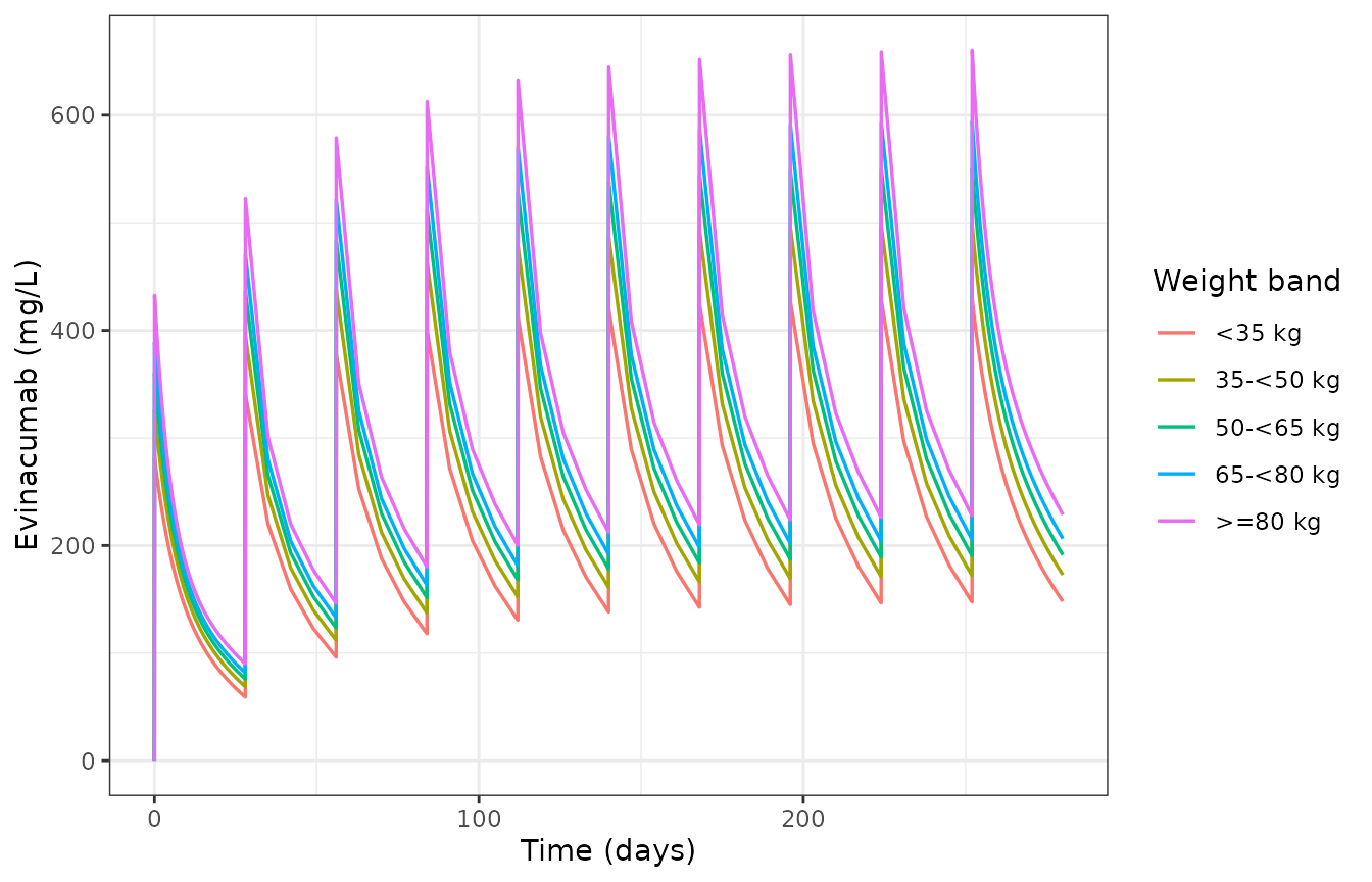
Typical-value evinacumab concentration and LDL-C over ten 15 mg/kg q4w infusions, by weight band. Compare with Figures S2 and S3 of Bihorel 2025.
ggplot(typ, aes(time, ldl, colour = band)) +
  geom_line(linewidth = 0.6) +
  labs(x = "Time (days)", y = "LDL-C (mg/dL)", colour = "Weight band") +
  theme_bw()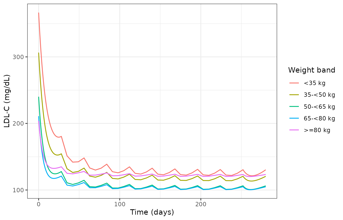
Typical-value evinacumab concentration and LDL-C over ten 15 mg/kg q4w infusions, by weight band. Compare with Figures S2 and S3 of Bihorel 2025.
Apheresis on top of treatment
The apheresis arm is time-varying, so it is driven by a covariate column that switches on for the duration of each session. Below, a patient on weekly 2.5-h apheresis is compared with the same patient without it.
aph_weekly <- function(tm) as.numeric((tm %% 7) < (2.5 / 24) & tm > 0)
fine <- sort(unique(c(seq(0, 84, by = 1 / 48), DOSE_T, DOSE_T + INF_D)))

with_aph <- solve_typ(make_subject(1, WT = 72, AGE = 43, times = fine,
                                   aph_fun = aph_weekly))
#> ℹ omega/sigma items treated as zero: 'etalcl', 'etalvc', 'etalka', 'etaltlag', 'etalrbase', 'etalkin', 'etalogitimax'
no_aph   <- solve_typ(make_subject(1, WT = 72, AGE = 43, times = fine))
#> ℹ omega/sigma items treated as zero: 'etalcl', 'etalvc', 'etalka', 'etaltlag', 'etalrbase', 'etalkin', 'etalogitimax'

cmp <- dplyr::bind_rows(
  dplyr::mutate(with_aph[with_aph$time <= 84, ], arm = "Evinacumab + weekly apheresis"),
  dplyr::mutate(no_aph[no_aph$time <= 84, ],     arm = "Evinacumab alone"))

ggplot(cmp, aes(time, ldl, colour = arm)) +
  geom_line(linewidth = 0.5) +
  labs(x = "Time (days)", y = "LDL-C (mg/dL)", colour = NULL) +
  theme_bw() + theme(legend.position = "top")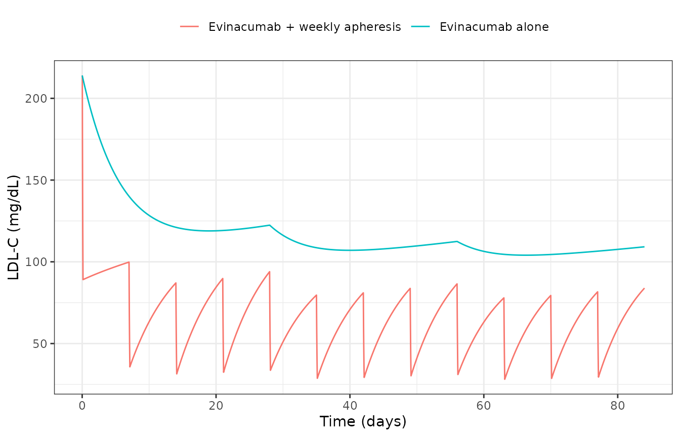
LDL-C with and without weekly 2.5-h lipoprotein apheresis, on a background of 15 mg/kg evinacumab q4w.
Assumptions and deviations
-
Infusion duration. The paper does not print the IV
infusion duration (the NONMEM dataset carries it in
DOSEDUR, which is not populated in the Table S2 sample). A 60-minute infusion is assumed here, per the approved labelling. Cmin and AUC are insensitive to this choice; only Cmax is affected, and it still lands within 2.5% of Table 4. - ANGPTL3 range. Figure 2 varies baseline ANGPTL3 between its observed minimum and maximum, which are not printed (Table 1 gives only mean 0.0914 and SD 0.0327 mg/L). Values of 0.03 and 0.20 mg/L are used here as plausible extremes; the assertion checks that the resulting ratios fall inside the paper’s stated 0.824-1.14 span rather than matching it exactly.
-
Age effect on %dLDL-C is not reproduced, and cannot
be. As shown above, steady-state %dLDL-C is algebraically
independent of
rbase, which is the only route by which age enters the model. This is a property of the published model, not of the transcription. The Discussion’s explanation invokes an age effect onVmaxthat the final model does not contain. -
Typical-value %dLDL-C runs below the Table 4
median. At the reference patient the model gives about 49-50%
versus a post hoc median of 58.0%. Two contributors: the Table 4 medians
are post hoc predictions over patients whose mean weight (67.9 kg in the
HoFH subset, Table 1) is below the 74.1 kg PK reference, and lower
weight raises
Imax; and %dLDL-C depends on where in the 28-day cycle LDL-C is sampled. No parameter was adjusted to close this gap. - Additive residual error for evinacumab. Table 2’s point estimate (0.0806 variance, i.e. 0.284 mg/L) sits well outside its own bootstrap 95% CI (0.00469-0.0214, i.e. 0.069-0.146 mg/L). The point estimate is used, as the published “Estimate” column, but the discrepancy is noted; it affects only residual-error simulation, not any structural prediction.
-
Race on
Imaxwas retained in the predecessor Pu 2021 model but formally removed here (Results 3.3), so it is documented incovariatesDataExcludedrather than implemented. -
Single-subject data override. Supplement Code 2
substitutes the observed baseline for one subject (
ID 244) and zeroesImaxfor four excluded outliers. These are data-handling exceptions specific to the original fit and are not reproduced in the packaged model. - Between-occasion variability is not present in the source model, and none is added.