PF-00821385 translational PK-PD (Langdon 2010)

Model and source

Langdon 2010 reports two parallel population PK-PD models for the discontinued HIV-1 gp120 cell-fusion inhibitor candidate PF-00821385 (Pfizer; molecular weight 440.49 g/mol):

Canine model (Langdon_2010_PF00821385_dog) – one-compartment PK with first-order oral absorption, fit to 88 oral and 22 IV plasma concentrations from 18 Beagle dogs at doses 0.5 - 120 mg/kg. PD describes heart rate (HR) as a baseline plus 24-hour cosine circadian rhythm plus a linear drug effect on free plasma concentration.
Human model (Langdon_2010_PF00821385_human) – two-compartment PK with first-order oral absorption, fit to 969 plasma concentrations from 24 healthy male volunteers receiving single ascending doses 3 - 1300 mg in the first-in- human study. PD describes supine pulse rate with the same baseline + circadian
- linear-drug-effect structure.

Both PD models use the slope on free drug concentration (bpm per uM unbound) so the species comparison is independent of plasma protein binding. The paper does not state the unbound fraction fu directly. In this package fu = 0.64 is FIXED via back-calculation from the canine 20 mg/kg toxicology Cmax data (see the Errata section). The same fu is used in both species because no species difference was reported.

dog_fn <- readModelDb("Langdon_2010_PF00821385_dog")
dog    <- dog_fn()
hum_fn <- readModelDb("Langdon_2010_PF00821385_human")
hum    <- hum_fn()

Canine reference: Langdon G, Davis JD, McFadyen LM, Dewhurst M, Brunton NS, Rawal JK, Van der Graaf PH, Benson N. Translational pharmacokinetic-pharmacodynamic modelling; application to cardiovascular safety data for PF-00821385, a novel HIV agent. Br J Clin Pharmacol. 2010 Apr;69(4):335-345. doi:10.1111/j.1365-2125.2009.03594.x.
Article: https://doi.org/10.1111/j.1365-2125.2009.03594.x (open-access on the Wiley journal landing page)

Population

The canine experiment used 18 Beagle dogs of similar weight (16.3 - 16.4 kg) from the Pfizer Sandwich laboratory colony. Four animals contributed the telemetric heart-rate data (vehicle plus 1.5, 5, 15 mg/kg PF-00821385 on separate occasions, with 96 fifteen-minute-binned HR observations per animal per dose) and 14 additional animals contributed satellite PK concentrations at 0.5, 20, 40, 100, and 120 mg/kg oral and 0.5 mg/kg IV. Cardiovascular telemetry was acquired via implanted Konigsberg pressure transducers and subcutaneous ECG electrodes.

The first-in-human study enrolled 24 healthy male volunteers aged 21 - 55 years with BMI 18 - 30 kg/m^2 in two single-ascending-dose cohorts of 12 (cohort 1: 3, 10, 30, 100 mg fasted; cohort 2: 250, 500, 1000, 1300 mg fasted plus a fed-state repeat of 500 mg). PK samples were drawn predose and at 0.5, 1, 1.5, 2, 3, 4, 6, 8, 12, 16, 24, 36 h post dose; supine pulse rate was recorded predose and at 1, 2, 4, 6, 8, 12, 24, 48 h. Morning dosing was performed at approximately 08:00. Dose escalation was gated by exposure- and HR-based stopping rules; the PD data set was correspondingly truncated, which limited the ability to fit an Emax-type concentration-response.

str(dog$meta$population)
#> List of 10
#>  $ species       : chr "beagle dog (Pfizer laboratory colony, conscious freely-moving)"
#>  $ n_subjects    : int 18
#>  $ n_studies     : int 1
#>  $ weight_range  : chr "16.3 - 16.4 kg"
#>  $ weight_median : chr "approximately 16.35 kg"
#>  $ sex_female_pct: num NA
#>  $ disease_state : chr "Healthy laboratory beagle (no induced disease)."
#>  $ dose_range    : chr "Oral gavage single doses 0.5, 1.5, 5, 15, 20, 40, 100, and 120 mg/kg. PD experiments (4 dogs): vehicle plus 1.5"| __truncated__
#>  $ regions       : chr "United Kingdom (Pfizer Sandwich laboratory colony)."
#>  $ notes         : chr "Cardiovascular telemetry data (heart rate, blood pressure) acquired as 1-minute means via implanted Konigsberg "| __truncated__
str(hum$meta$population)
#> List of 11
#>  $ species       : chr "human"
#>  $ n_subjects    : int 24
#>  $ n_studies     : int 1
#>  $ age_range     : chr "21 - 55 years"
#>  $ weight_range  : chr "> 50 kg"
#>  $ sex_female_pct: num 0
#>  $ race_ethnicity: NULL
#>  $ disease_state : chr "Healthy adult male volunteers (no diagnosed condition)."
#>  $ dose_range    : chr "Single ascending oral suspension doses, two cohorts of 12 volunteers each. Cohort 1 (fasted): 3, 10, 30, 100 mg"| __truncated__
#>  $ regions       : chr "Singapore (Singapore General Hospital)."
#>  $ notes         : chr "Body mass index approximately 18 - 30 kg/m^2 per inclusion criteria. Plasma PK samples at predose and 0.5, 1, 1"| __truncated__

Source trace

Per-parameter origin is recorded as in-file comments next to each ini() entry in the two model files. The tables below collect the source location for every model element in one place.

Canine model (`Langdon_2010_PF00821385_dog`)

Equation / parameter	Value	Source location
PK structural form: 1-cmt with first-order oral absorption	n/a	Methods, Canine PK-PD analysis paragraph 2; Table 1 footer
PD structural form: baseline + 24-h cosine + linear drug effect (Eqs. 1 + 2)	n/a	Methods, Canine PK-PD analysis Equations 1 and 2 (page 338)
`lfdepot = log(1.01)` -> F = 1.01	1.01	Table 1: F = 1.01 (SE 0.003; 95% CI 1.00 - 1.02)
`lka = log(2.42)` -> ka = 2.42 1/h	2.42	Table 1: ka = 2.42 1/h (SE 0.520; 95% CI 1.40 - 3.44)
`lcl = log(1.02)` -> CL/F = 1.02 L/h	1.02	Table 1: CL/F = 1.02 L/h (SE 0.135; 95% CI 0.755 - 1.28)
`lvc = log(7.05)` -> V/F = 7.05 L	7.05	Table 1: V/F = 7.05 L (SE 0.640; 95% CI 5.80 - 8.30)
`lbase = log(68.2)` -> BASE = 68.2 bpm	68.2	Table 1: BASE = 68.2 bpm
`lamp = log(12.4)` -> AMP = 12.4 bpm	12.4	Table 1: AMP = 12.4 bpm
`lpeak = log(10.4)` -> PEAK = 10.4 h	10.4	Table 1: PEAK = 10.4 h
`lslope = log(1.76)` -> SLOPE = 1.76 bpm/uM free	1.76	Table 1: SLOPE = 1.76 bpm/uM-free; Results “the typical drug effect was 1.76 bpm mM-1 (95% CI 1.17, 2.35) free drug”
`lfu = fixed(log(0.64))` -> fu = 0.64	0.64	Back-calculated from Introduction (see Errata)
`etalka ~ 0.404`	0.404	Table 1: Variance for ka (95% CI 0.128 - 0.680)
`etalcl ~ 0.311`	0.311	Table 1: Variance for CL/F (95% CI 0.111 - 0.511)
`etalvc ~ 0.136`	0.136	Table 1: Variance for V/F (95% CI 0.003 - 0.269)
`etalbase ~ 0.0057`	0.0057	Table 1: Variance for BASE (95% CI 0.0024 - 0.0090)
`etalpeak ~ 0.0134`	0.0134	Table 1: Variance for PEAK (95% CI 0.0044 - 0.0224)
`propSd = 0.181`	0.181	Table 1: PK proportional residual error
`addSd = 9.43` ng/mL	9.43	Table 1: PK additive residual error
`addSd_HR = 14.1` bpm	14.1	Table 1: PD additive residual error

Human model (`Langdon_2010_PF00821385_human`)

Equation / parameter	Value	Source location
PK structural form: 2-cmt with first-order oral absorption	n/a	Methods, Human PK-PD analysis paragraph 1
PD structural form: baseline + 24-h cosine + linear drug effect (Eqs. 1 + 2)	n/a	Methods, Human PK-PD analysis paragraph 2; Eqs. 1 and 2 reused from page 338
`lfdepot = fixed(log(1))` -> F = 1 (FIXED)	1	Table 2: F = 1 (FIXED)
`lka = log(0.599)` -> ka = 0.599 1/h	0.599	Table 2: ka = 0.599 1/h (95% CI 0.582 - 0.616)
`lcl = log(36.7)` -> CL/F = 36.7 L/h	36.7	Table 2: CL/F = 36.7 L/h (95% CI 32.8 - 40.9)
`lvc = log(18.4)` -> Vc/F = 18.4 L	18.4	Table 2: Vc/F = 18.4 L (95% CI 14.2 - 24.3)
`lvp = log(6.88)` -> Vp/F = 6.88 L	6.88	Table 2: Vp/F = 6.88 L (95% CI 5.51 - 8.89)
`lq = log(0.704)` -> Q/F = 0.704 L/h	0.704	Table 2: Q = 0.704 L/h (95% CI 0.546 - 0.945)
`lbase = log(61.5)` -> BASE = 61.5 bpm	61.5	Table 2: BASE = 61.5 bpm
`lamp = log(4.01)` -> AMP = 4.01 bpm	4.01	Table 2: AMP = 4.01 bpm
`lpeak = log(14.3)` -> PEAK = 14.3 h	14.3	Table 2: PEAK = 14.3 h
`lslope = log(0.76)` -> SLOPE = 0.76 bpm/uM free	0.76	Table 2: SLOPE = 0.76 bpm/uM-free; Results “the drug effect is 0.76 bpm mM-1 (95% CI 0.54, 1.14) free drug”
`lfu = fixed(log(0.64))` -> fu = 0.64	0.64	Back-calculated from Introduction (see Errata)
`etalfdepot ~ 0.075`	0.075	Table 2: Variance for F (95% CI 0.017 - 0.123)
`etalcl ~ 0.039`	0.039	Table 2: Variance for CL (95% CI degenerate; see Errata)
`etalvc ~ 0.332`	0.332	Table 2: Variance for Vc (95% CI 0.164 - 0.505)
`etalbase ~ 0.0094`	0.0094	Table 2: Variance for BASE (95% CI 0.0050 - 0.0133)
`etalpeak ~ 0.0206`	0.0206	Table 2: Variance for PEAK (95% CI 0.0099 - 0.0299)
`expSd = 0.658`	0.658	Table 2: PK residual error (Methods: “additive error on the log-transformed concentrations”)
`addSd_HR = 4.77` bpm	4.77	Table 2: PD additive residual error

Parameter table (paper vs. file)

dog_ini <- dog$iniDf
dog_tab <- data.frame(
  parameter = c("F", "CL/F (L/h)", "V/F (L)", "ka (1/h)",
                "BASE (bpm)", "AMP (bpm)", "PEAK (h)", "SLOPE (bpm/uM free)"),
  paper_T1  = c("1.01 (1.00 - 1.02)", "1.02 (0.755 - 1.28)",
                "7.05 (5.80 - 8.30)", "2.42 (1.40 - 3.44)",
                "68.2 (66.2 - 70.2)", "12.4 (11.0 - 13.8)",
                "10.4 (9.91 - 10.88)", "1.76 (1.17 - 2.35)"),
  packaged  = c(
    sprintf("%.3f", exp(dog_ini$est[dog_ini$name == "lfdepot"])),
    sprintf("%.3f", exp(dog_ini$est[dog_ini$name == "lcl"])),
    sprintf("%.2f", exp(dog_ini$est[dog_ini$name == "lvc"])),
    sprintf("%.2f", exp(dog_ini$est[dog_ini$name == "lka"])),
    sprintf("%.1f", exp(dog_ini$est[dog_ini$name == "lbase"])),
    sprintf("%.1f", exp(dog_ini$est[dog_ini$name == "lamp"])),
    sprintf("%.1f", exp(dog_ini$est[dog_ini$name == "lpeak"])),
    sprintf("%.2f", exp(dog_ini$est[dog_ini$name == "lslope"]))
  )
)
knitr::kable(dog_tab,
             caption = "Canine model: Langdon 2010 Table 1 paper values vs. packaged ini() values. Paper values are point estimates with 95% CI in parentheses.")

Canine model: Langdon 2010 Table 1 paper values vs. packaged ini() values. Paper values are point estimates with 95% CI in parentheses.
parameter	paper_T1	packaged
F	1.01 (1.00 - 1.02)	1.010
CL/F (L/h)	1.02 (0.755 - 1.28)	1.020
V/F (L)	7.05 (5.80 - 8.30)	7.05
ka (1/h)	2.42 (1.40 - 3.44)	2.42
BASE (bpm)	68.2 (66.2 - 70.2)	68.2
AMP (bpm)	12.4 (11.0 - 13.8)	12.4
PEAK (h)	10.4 (9.91 - 10.88)	10.4
SLOPE (bpm/uM free)	1.76 (1.17 - 2.35)	1.76

hum_ini <- hum$iniDf
hum_tab <- data.frame(
  parameter = c("F", "CL/F (L/h)", "Vc/F (L)", "Vp/F (L)", "Q/F (L/h)",
                "ka (1/h)", "BASE (bpm)", "AMP (bpm)", "PEAK (h)",
                "SLOPE (bpm/uM free)"),
  paper_T2  = c("1 (FIXED)", "36.7 (32.8 - 40.9)", "18.4 (14.2 - 24.3)",
                "6.88 (5.51 - 8.89)", "0.704 (0.546 - 0.945)",
                "0.599 (0.582 - 0.616)", "61.5 (59.3 - 63.6)",
                "4.01 (3.33 - 4.82)", "14.3 (13.3 - 15.2)",
                "0.76 (0.54 - 1.14)"),
  packaged  = c(
    sprintf("%.2f", exp(hum_ini$est[hum_ini$name == "lfdepot"])),
    sprintf("%.2f", exp(hum_ini$est[hum_ini$name == "lcl"])),
    sprintf("%.2f", exp(hum_ini$est[hum_ini$name == "lvc"])),
    sprintf("%.2f", exp(hum_ini$est[hum_ini$name == "lvp"])),
    sprintf("%.3f", exp(hum_ini$est[hum_ini$name == "lq"])),
    sprintf("%.3f", exp(hum_ini$est[hum_ini$name == "lka"])),
    sprintf("%.1f", exp(hum_ini$est[hum_ini$name == "lbase"])),
    sprintf("%.2f", exp(hum_ini$est[hum_ini$name == "lamp"])),
    sprintf("%.1f", exp(hum_ini$est[hum_ini$name == "lpeak"])),
    sprintf("%.2f", exp(hum_ini$est[hum_ini$name == "lslope"]))
  )
)
knitr::kable(hum_tab,
             caption = "Human model: Langdon 2010 Table 2 paper values vs. packaged ini() values. Paper values are point estimates with bootstrap 95% CI in parentheses.")

Human model: Langdon 2010 Table 2 paper values vs. packaged ini() values. Paper values are point estimates with bootstrap 95% CI in parentheses.
parameter	paper_T2	packaged
F	1 (FIXED)	1.00
CL/F (L/h)	36.7 (32.8 - 40.9)	36.70
Vc/F (L)	18.4 (14.2 - 24.3)	18.40
Vp/F (L)	6.88 (5.51 - 8.89)	6.88
Q/F (L/h)	0.704 (0.546 - 0.945)	0.704
ka (1/h)	0.599 (0.582 - 0.616)	0.599
BASE (bpm)	61.5 (59.3 - 63.6)	61.5
AMP (bpm)	4.01 (3.33 - 4.82)	4.01
PEAK (h)	14.3 (13.3 - 15.2)	14.3
SLOPE (bpm/uM free)	0.76 (0.54 - 1.14)	0.76

Canine simulation – Figure 1 replication

The four PD dose levels (vehicle, 1.5, 5, 15 mg/kg) were administered to the 4 Beagle dogs at 09:00. With cohort weight approximately 16.3 kg, the per- animal doses are 24.4, 81.5, and 244.5 mg respectively.

set.seed(20100401L)
n_per_dose_dog <- 30L
wt_dog <- 16.3                                                     # cohort mean kg
dose_levels_dog <- c(vehicle = 0, "1.5 mg/kg" = 1.5,
                     "5 mg/kg" = 5, "15 mg/kg" = 15)               # mg/kg
amts_dog <- dose_levels_dog * wt_dog                                # mg

times_dog <- c(seq(0, 12, by = 0.25), seq(12.5, 24, by = 0.5))

make_dog_cohort <- function(amt_mg, label, n_sub, id_offset) {
  ids <- id_offset + seq_len(n_sub)
  dose_rows <- data.frame(
    id        = ids,
    time      = 0,
    amt       = amt_mg,
    evid      = 1L,
    cmt       = "depot",
    treatment = label
  )
  obs_rows <- expand.grid(id = ids, time = times_dog,
                          KEEP.OUT.ATTRS = FALSE)
  obs_rows$amt       <- 0
  obs_rows$evid      <- 0L
  obs_rows$cmt       <- "HR"
  obs_rows$treatment <- label
  rbind(dose_rows, obs_rows[order(obs_rows$id, obs_rows$time), ])
}

events_dog <- bind_rows(
  make_dog_cohort(amts_dog[1], names(dose_levels_dog)[1], n_per_dose_dog,   0L),
  make_dog_cohort(amts_dog[2], names(dose_levels_dog)[2], n_per_dose_dog,  30L),
  make_dog_cohort(amts_dog[3], names(dose_levels_dog)[3], n_per_dose_dog,  60L),
  make_dog_cohort(amts_dog[4], names(dose_levels_dog)[4], n_per_dose_dog,  90L)
)
#> Warning in data.frame(id = ids, time = 0, amt = amt_mg, evid = 1L, cmt =
#> "depot", : row names were found from a short variable and have been discarded
#> Warning in data.frame(id = ids, time = 0, amt = amt_mg, evid = 1L, cmt =
#> "depot", : row names were found from a short variable and have been discarded
#> Warning in data.frame(id = ids, time = 0, amt = amt_mg, evid = 1L, cmt =
#> "depot", : row names were found from a short variable and have been discarded
#> Warning in data.frame(id = ids, time = 0, amt = amt_mg, evid = 1L, cmt =
#> "depot", : row names were found from a short variable and have been discarded
stopifnot(!anyDuplicated(unique(events_dog[, c("id", "time", "evid")])))

sim_dog <- rxode2::rxSolve(
  dog,
  events     = events_dog,
  keep       = c("treatment"),
  returnType = "data.frame"
)

sim_dog |>
  filter(time > 0) |>
  group_by(time, treatment) |>
  summarise(
    Q05 = quantile(HR, 0.05, na.rm = TRUE),
    Q50 = quantile(HR, 0.50, na.rm = TRUE),
    Q95 = quantile(HR, 0.95, na.rm = TRUE),
    .groups = "drop"
  ) |>
  mutate(treatment = factor(treatment, levels = names(dose_levels_dog))) |>
  ggplot(aes(time, Q50)) +
  geom_ribbon(aes(ymin = Q05, ymax = Q95), alpha = 0.25, fill = "#1f77b4") +
  geom_line(linewidth = 0.7, colour = "#1f77b4") +
  facet_wrap(~ treatment, ncol = 2) +
  labs(x = "Time after dose (h)", y = "Heart rate (bpm)",
       title = "Canine heart rate VPC",
       caption = "Replicates Figure 1 of Langdon 2010 (vehicle, 1.5, 5, 15 mg/kg PD doses).") +
  theme_minimal()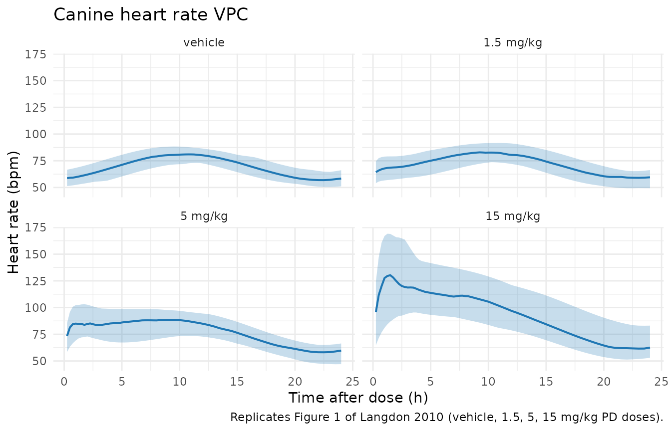

Simulated VPC of canine heart rate vs. time after the morning dose, replicating Figure 1 of Langdon 2010. Median and 5 - 95 percentile bands; n = 30 simulated dogs per dose group.

sim_dog |>
  filter(time > 0, treatment != "vehicle") |>
  group_by(time, treatment) |>
  summarise(
    Q05 = quantile(Cc, 0.05, na.rm = TRUE),
    Q50 = quantile(Cc, 0.50, na.rm = TRUE),
    Q95 = quantile(Cc, 0.95, na.rm = TRUE),
    .groups = "drop"
  ) |>
  filter(Q50 > 0) |>
  mutate(treatment = factor(treatment, levels = names(dose_levels_dog))) |>
  ggplot(aes(time, Q50)) +
  geom_ribbon(aes(ymin = pmax(Q05, 1e-3), ymax = Q95),
              alpha = 0.25, fill = "#d62728") +
  geom_line(linewidth = 0.7, colour = "#d62728") +
  facet_wrap(~ treatment, ncol = 3) +
  scale_y_log10() +
  labs(x = "Time after dose (h)", y = "PF-00821385 plasma Cc (ng/mL)",
       title = "Canine plasma PF-00821385 VPC") +
  theme_minimal()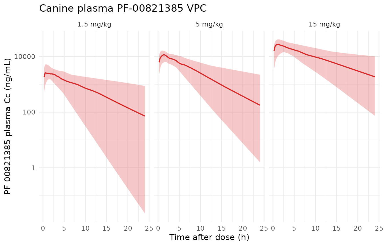

Simulated canine PF-00821385 plasma concentrations on a log scale for the PD-dose-range cohorts.

Human simulation – Figure 3 replication

Single ascending doses 3, 10, 30, 100, 250, 500, 1000, 1300 mg in healthy volunteers (08:00 morning dose). The vignette simulates 30 subjects per dose group; the original FIH study had only ~9 subjects per dose group in the oral-suspension treatment arms.

set.seed(20100501L)
n_per_dose_hum <- 30L
doses_hum <- c(3, 10, 30, 100, 250, 500, 1000, 1300)               # mg

times_hum <- c(seq(0, 12, by = 0.25), seq(13, 48, by = 0.5))

make_hum_cohort <- function(amt_mg, n_sub, id_offset) {
  label <- sprintf("%d mg", amt_mg)
  ids   <- id_offset + seq_len(n_sub)
  dose_rows <- data.frame(
    id        = ids,
    time      = 0,
    amt       = amt_mg,
    evid      = 1L,
    cmt       = "depot",
    treatment = label
  )
  obs_rows <- expand.grid(id = ids, time = times_hum,
                          KEEP.OUT.ATTRS = FALSE)
  obs_rows$amt       <- 0
  obs_rows$evid      <- 0L
  obs_rows$cmt       <- "HR"
  obs_rows$treatment <- label
  rbind(dose_rows, obs_rows[order(obs_rows$id, obs_rows$time), ])
}

events_hum <- bind_rows(lapply(seq_along(doses_hum), function(i) {
  make_hum_cohort(doses_hum[i], n_per_dose_hum, id_offset = (i - 1L) * 100L)
}))
stopifnot(!anyDuplicated(unique(events_hum[, c("id", "time", "evid")])))

sim_hum <- rxode2::rxSolve(
  hum,
  events     = events_hum,
  keep       = c("treatment"),
  returnType = "data.frame"
)

treatment_levels <- sprintf("%d mg", doses_hum)
sim_hum |>
  filter(time > 0) |>
  group_by(time, treatment) |>
  summarise(
    Q05 = quantile(HR, 0.05, na.rm = TRUE),
    Q50 = quantile(HR, 0.50, na.rm = TRUE),
    Q95 = quantile(HR, 0.95, na.rm = TRUE),
    .groups = "drop"
  ) |>
  mutate(treatment = factor(treatment, levels = treatment_levels)) |>
  ggplot(aes(time, Q50)) +
  geom_ribbon(aes(ymin = Q05, ymax = Q95), alpha = 0.25, fill = "#2ca02c") +
  geom_line(linewidth = 0.6, colour = "#2ca02c") +
  facet_wrap(~ treatment, ncol = 4) +
  labs(x = "Time after dose (h)", y = "Supine pulse rate (bpm)",
       title = "Human supine pulse-rate VPC across the FIH dose range",
       caption = "Replicates the right panels of Figure 3 of Langdon 2010 (10 - 1300 mg single ascending doses).") +
  theme_minimal()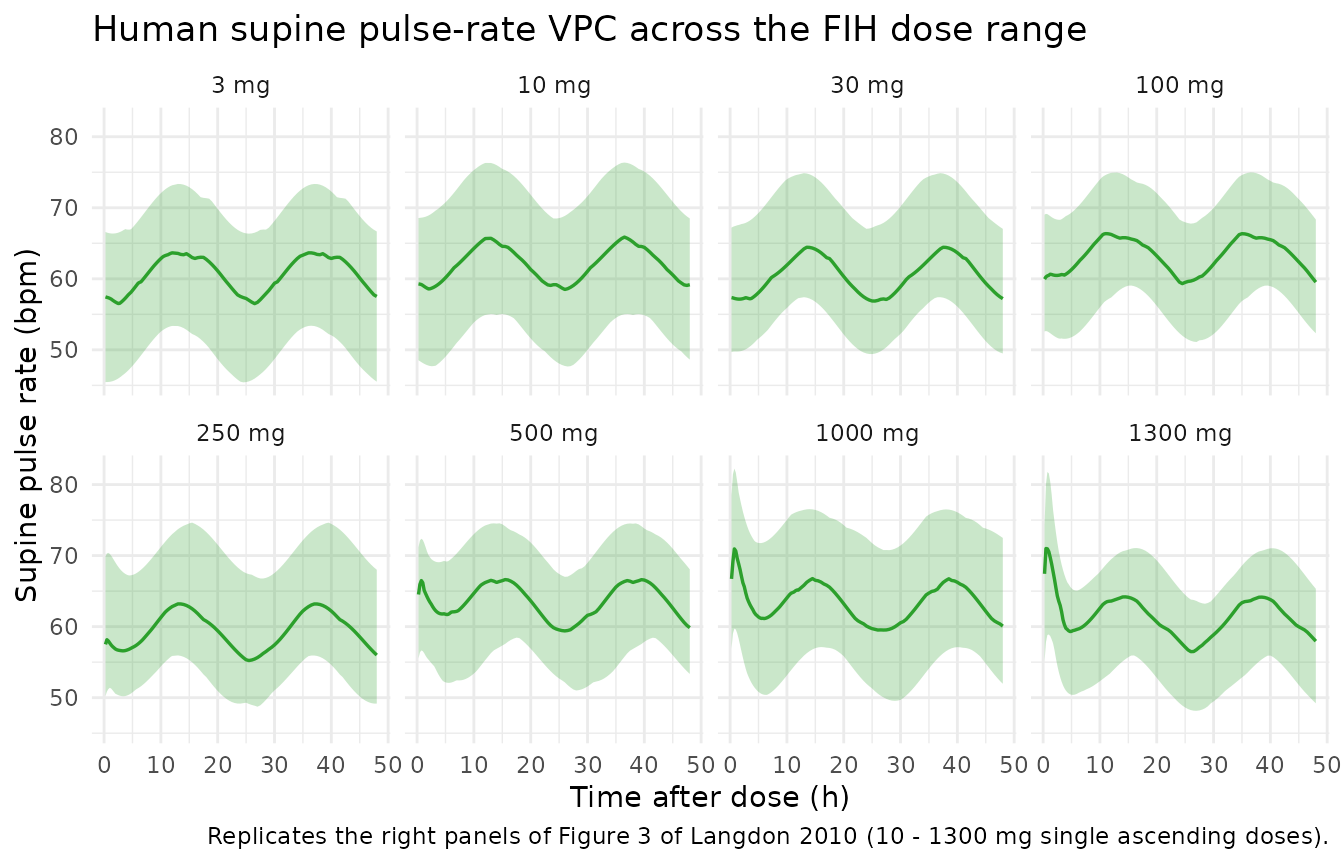

Simulated VPC of human supine pulse rate vs. time after the morning dose across the FIH single-ascending-dose range. Median and 5 - 95 percentile bands; n = 30 simulated subjects per dose group.

sim_hum |>
  filter(time > 0) |>
  group_by(time, treatment) |>
  summarise(
    Q05 = quantile(Cc, 0.05, na.rm = TRUE),
    Q50 = quantile(Cc, 0.50, na.rm = TRUE),
    Q95 = quantile(Cc, 0.95, na.rm = TRUE),
    .groups = "drop"
  ) |>
  filter(Q50 > 0) |>
  mutate(treatment = factor(treatment, levels = treatment_levels)) |>
  ggplot(aes(time, Q50)) +
  geom_ribbon(aes(ymin = pmax(Q05, 1), ymax = Q95),
              alpha = 0.25, fill = "#9467bd") +
  geom_line(linewidth = 0.6, colour = "#9467bd") +
  geom_hline(yintercept = 28400, linetype = "dashed", colour = "grey40") +
  facet_wrap(~ treatment, ncol = 4) +
  scale_y_log10() +
  labs(x = "Time after dose (h)", y = "PF-00821385 plasma Cc (ng/mL)",
       title = "Human plasma PF-00821385 VPC") +
  theme_minimal()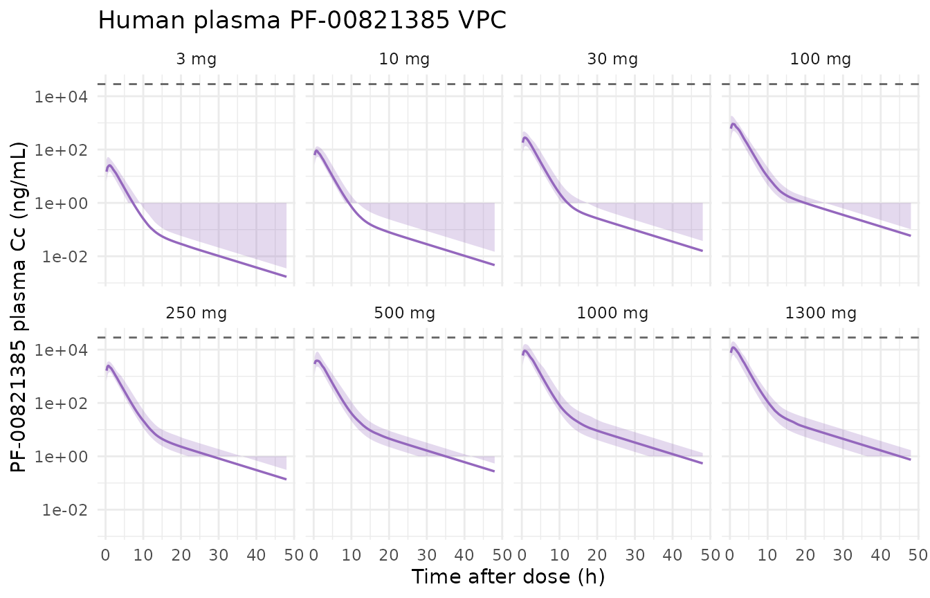

Simulated human PF-00821385 plasma concentrations on a log scale across the FIH dose range. The 28400 ng/mL dose-escalation stopping threshold (Methods ‘First-in-human study design’) is drawn as a horizontal reference line.

Concentration-response (Figure 4 replication)

Figure 4 of Langdon 2010 plots heart-rate change versus free PF-00821385 plasma concentration in both species. The typical-value drug-effect lines are encoded directly in the packaged models (SLOPE = 1.76 bpm/uM-free for dog and SLOPE = 0.76 bpm/uM-free for human) and shown below.

free_grid <- tibble(
  Cc_free_uM = seq(0, 80, by = 0.5)
)
fig4 <- bind_rows(
  free_grid |> mutate(species = "Beagle dog",
                      dHR     = 1.76 * Cc_free_uM),
  free_grid |> mutate(species = "Human",
                      dHR     = 0.76 * Cc_free_uM)
)
ggplot(fig4, aes(Cc_free_uM, dHR, colour = species)) +
  geom_line(linewidth = 0.8) +
  scale_colour_manual(values = c("Beagle dog" = "#1f77b4",
                                 "Human"      = "#2ca02c")) +
  labs(x = "Free PF-00821385 concentration (uM)",
       y = "Heart-rate change from baseline (bpm)",
       colour = NULL,
       title = "PF-00821385 concentration-response",
       caption = "Replicates Figure 4 of Langdon 2010 (linear drug-effect lines).") +
  theme_minimal() +
  theme(legend.position = "bottom")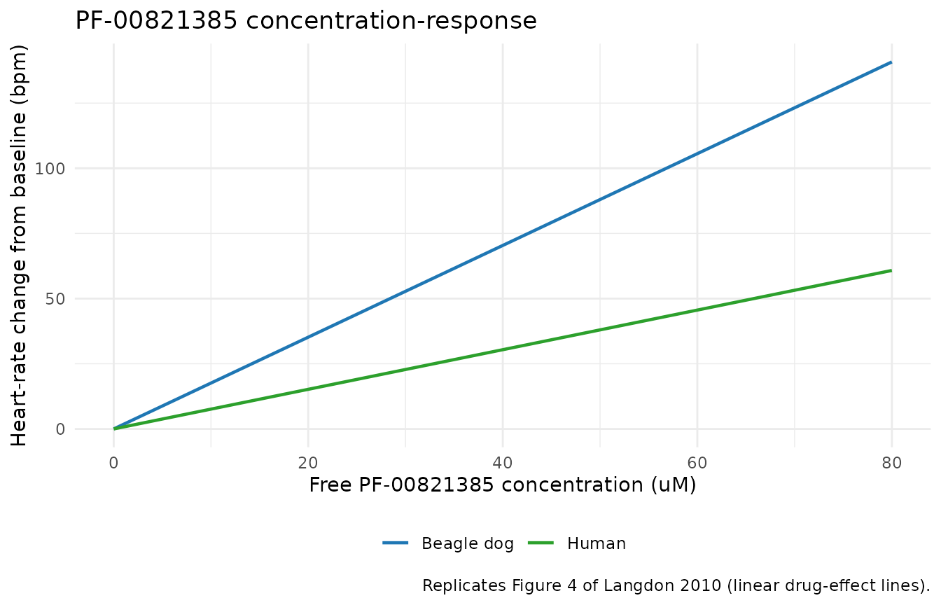

Typical-value heart-rate change vs. free plasma concentration for the canine and human PD models. SLOPE values are reproduced from Langdon 2010 Tables 1 and 2.

PKNCA validation

The source publication does not report a tabulated NCA summary (Tables 1 and 2 list popPK parameters, not NCA). PKNCA-derived Cmax, Tmax, AUC, and half-life are useful as internal sanity checks against the population PK estimates and against the paper’s first-in-human dose-escalation stopping criterion of mean peak total plasma concentrations exceeding 28400 ng/mL.

Canine NCA

dog_nca_input <- sim_dog |>
  filter(treatment != "vehicle") |>
  dplyr::filter(!is.na(Cc)) |>
  dplyr::select(id, time, Cc, treatment)

dog_nca_input <- dplyr::bind_rows(
  dog_nca_input,
  dog_nca_input |> dplyr::distinct(id, treatment) |>
    dplyr::mutate(time = 0, Cc = 0)
) |>
  dplyr::distinct(id, treatment, time, .keep_all = TRUE) |>
  dplyr::arrange(id, treatment, time)

dog_dose_df <- events_dog |>
  filter(evid == 1, treatment != "vehicle") |>
  select(id, time, amt, treatment)

dog_conc_obj <- PKNCA::PKNCAconc(dog_nca_input,
                                 Cc ~ time | treatment + id,
                                 concu = "ng/mL", timeu = "h")
dog_dose_obj <- PKNCA::PKNCAdose(dog_dose_df,
                                 amt ~ time | treatment + id,
                                 doseu = "mg")

dog_intervals <- data.frame(
  start       = 0,
  end         = Inf,
  cmax        = TRUE,
  tmax        = TRUE,
  aucinf.obs  = TRUE,
  half.life   = TRUE
)
dog_nca_res <- PKNCA::pk.nca(PKNCA::PKNCAdata(dog_conc_obj, dog_dose_obj,
                                              intervals = dog_intervals))

dog_nca_summary <- as.data.frame(dog_nca_res$result) |>
  group_by(treatment, PPTESTCD) |>
  summarise(median = median(PPORRES, na.rm = TRUE), .groups = "drop") |>
  tidyr::pivot_wider(names_from = PPTESTCD, values_from = median) |>
  mutate(treatment = factor(treatment,
                            levels = c("1.5 mg/kg", "5 mg/kg", "15 mg/kg"))) |>
  arrange(treatment)
knitr::kable(dog_nca_summary,
             caption = "Canine simulated PKNCA per-dose summary (median across 30 simulated subjects).")

Canine simulated PKNCA per-dose summary (median across 30 simulated subjects).
treatment	adj.r.squared	aucinf.obs	clast.obs	clast.pred	cmax	half.life	lambda.z	lambda.z.n.points	lambda.z.time.first	lambda.z.time.last	r.squared	span.ratio	tlast	tmax
1.5 mg/kg	0.9999817	21971.94	72.36008	72.67226	2635.292	4.152303	0.1676071	68	1.25	24	0.9999820	5.589841	24	1.00
5 mg/kg	0.9999625	80607.69	177.80700	178.19255	11841.616	3.785008	0.1831763	67	1.50	24	0.9999630	5.879767	24	1.25
15 mg/kg	0.9999808	249096.15	1857.99441	1864.31307	27908.971	5.443481	0.1273603	67	1.50	24	0.9999811	4.130359	24	1.25

Human NCA

hum_nca_input <- sim_hum |>
  dplyr::filter(!is.na(Cc)) |>
  dplyr::select(id, time, Cc, treatment)

hum_nca_input <- dplyr::bind_rows(
  hum_nca_input,
  hum_nca_input |> dplyr::distinct(id, treatment) |>
    dplyr::mutate(time = 0, Cc = 0)
) |>
  dplyr::distinct(id, treatment, time, .keep_all = TRUE) |>
  dplyr::arrange(id, treatment, time)

hum_dose_df <- events_hum |>
  filter(evid == 1) |>
  select(id, time, amt, treatment)

hum_conc_obj <- PKNCA::PKNCAconc(hum_nca_input,
                                 Cc ~ time | treatment + id,
                                 concu = "ng/mL", timeu = "h")
hum_dose_obj <- PKNCA::PKNCAdose(hum_dose_df,
                                 amt ~ time | treatment + id,
                                 doseu = "mg")

hum_intervals <- data.frame(
  start       = 0,
  end         = Inf,
  cmax        = TRUE,
  tmax        = TRUE,
  aucinf.obs  = TRUE,
  half.life   = TRUE
)
hum_nca_res <- PKNCA::pk.nca(PKNCA::PKNCAdata(hum_conc_obj, hum_dose_obj,
                                              intervals = hum_intervals))

hum_nca_summary <- as.data.frame(hum_nca_res$result) |>
  group_by(treatment, PPTESTCD) |>
  summarise(median = median(PPORRES, na.rm = TRUE), .groups = "drop") |>
  tidyr::pivot_wider(names_from = PPTESTCD, values_from = median) |>
  mutate(treatment = factor(treatment,
                            levels = sprintf("%d mg", doses_hum))) |>
  arrange(treatment)
knitr::kable(hum_nca_summary,
             caption = "Human simulated PKNCA per-dose summary (median across 30 simulated subjects).")

Human simulated PKNCA per-dose summary (median across 30 simulated subjects).
treatment	adj.r.squared	aucinf.obs	clast.obs	clast.pred	cmax	half.life	lambda.z	lambda.z.n.points	lambda.z.time.first	lambda.z.time.last	r.squared	span.ratio	tlast	tmax
3 mg	0.9999217	79.01062	0.0017058	0.0016952	26.02000	6.868797	0.1009125	62	17.5	48	0.9999230	4.440371	48	1.00
10 mg	0.9999245	239.57737	0.0046654	0.0046371	93.69206	6.857097	0.1010846	62	17.5	48	0.9999257	4.442495	48	0.75
30 mg	0.9999161	816.84236	0.0158140	0.0157135	283.12893	6.863764	0.1009865	62	17.5	48	0.9999175	4.420811	48	0.75
100 mg	0.9999176	2787.49039	0.0584670	0.0581143	952.20836	6.862766	0.1010011	62	17.5	48	0.9999189	4.436466	48	0.75
250 mg	0.9999199	6753.38898	0.1366552	0.1357923	2505.65786	6.864715	0.1009725	62	17.5	48	0.9999212	4.440690	48	0.75
500 mg	0.9999212	12246.19246	0.2720998	0.2705571	3915.73659	6.876505	0.1007993	62	17.5	48	0.9999225	4.439026	48	1.00
1000 mg	0.9999157	26197.38722	0.5426274	0.5390559	9154.80414	6.857259	0.1010822	62	17.5	48	0.9999171	4.443450	48	0.75
1300 mg	0.9999261	35974.98858	0.7453548	0.7407548	12187.32532	6.866225	0.1009503	62	17.5	48	0.9999273	4.436873	48	0.75

The simulated median Cmax at 1300 mg should sit near the published 28400 ng/mL stopping threshold (the paper truncated dose escalation when the threshold was approached).

Assumptions and deviations

Plasma unbound fraction fu was not reported. The paper expresses the PD slope in units of bpm per uM free PF-00821385 but does not state the unbound fraction used internally in NONMEM. The package fixes fu = 0.64 via back-calculation from the canine 20 mg/kg single-dose toxicology datum in the Introduction (“unbound Cmax = 56 uM at 20 mg/kg”): with the Table 1 typical-value PK parameters (D = 326 mg, F = 1.01, ka = 2.42, V/F = 7.05, CL/F = 1.02, kel = 0.145), the predicted total Cmax is 38.7 mg/L = 87.8 uM total, giving fu = 56 / 87.8 = 0.64. The same fu is applied to both species because no species difference was reported. Operator-confirmed via sidecar 2026-06-17 (see tracking/operator_followups.md if open). PF-00821385 development was discontinued at first-in-human (paper Conclusion: “further development of PF-00821385 will not be pursued”), so author correspondence is unlikely to recover the original NONMEM value. A user with access to a different fu measurement can override lfu at simulation time.
Canine text-table discrepancy on PD IIV. The Methods text states “IIV was included on the following structural parameters: baseline HR and amplitude of the circadian effect” but Table 1 reports variance terms for BASE and PEAK (not AMP). The package follows Table 1 (IIV on BASE and PEAK) because Table 1 carries the authoritative final parameter values; the text is interpreted as an editorial inconsistency.
Human CL IIV bootstrap CI is degenerate. Table 2 reports a point estimate Variance for CL = 0.039 with bootstrap 95% CI [8.73e-9, 9.35e-4]. The CI upper bound is two orders of magnitude smaller than the point estimate, implying that the bootstrap could not reliably identify a positive variance from the 24-subject FIH dataset. The package retains the NONMEM point estimate 0.039 (CV approximately 20%) as the authoritative IIV magnitude; a user reproducing the simulated marginal distributions may prefer to set etalcl ~ 0 to match the bootstrap-implied near-zero variance.
Human PK residual is log-additive, dimensionless. Table 2 lists “PK residual error (ng/mL) 0.658” but Methods state “residual variability was modelled as an additive error on the log-transformed concentrations”. The Table 2 unit annotation ng/mL is interpreted as an editorial inconsistency; the value 0.658 is the log-scale additive SD (dimensionless), encoded in the package as expSd <- 0.658 with Cc ~ lnorm(expSd).
Bioavailability F in the human model. Table 2 reports F = 1 (FIXED) at the population level but a Variance for F = 0.075. The package encodes lfdepot <- fixed(log(1)) together with etalfdepot ~ 0.075 so the population value is anchored at 1 while individual F values vary log- normally; this matches the standard NONMEM “fix population, estimate IIV” pattern.
PK and PD parameters were fit sequentially in the source. Individual Bayesian post hoc PK estimates served as input to the PD fit (Methods paragraph ‘Canine PK-PD analysis’ and ‘Human PK-PD analysis’). In the packaged model the PK and PD layers are integrated so a single simulation exposes both concentration and HR trajectories; users replicating the original sequential fit should re-fit the PK and PD layers separately.
Dose units. The dog model takes doses in mg per event row. The paper reports dog doses as mg/kg; the vignette converts using a cohort body weight of 16.3 kg. The human model takes doses in mg directly.
Doses at 09:00 (dog) / 08:00 (human). The cosine circadian rhythm centres PEAK on time after the morning dose (10.4 h for dog, 14.3 h for human). Users simulating a different dosing time should shift the event-table time origin accordingly.