Gentamicin (Llanos 2017)
Source:vignettes/articles/Llanos_2017_gentamicin.Rmd
Llanos_2017_gentamicin.Rmd
library(nlmixr2lib)
library(PKNCA)
#>
#> Attaching package: 'PKNCA'
#> The following object is masked from 'package:stats':
#>
#>     filter
library(rxode2)
#> rxode2 5.1.2 using 2 threads (see ?getRxThreads)
#>   no cache: create with `rxCreateCache()`
library(dplyr)
#>
#> Attaching package: 'dplyr'
#> The following objects are masked from 'package:stats':
#>
#>     filter, lag
#> The following objects are masked from 'package:base':
#>
#>     intersect, setdiff, setequal, union
library(tidyr)
library(ggplot2)
Model and source
- Citation: Llanos-Paez CC, Staatz CE, Lawson R, Hennig S. A Population Pharmacokinetic Model of Gentamicin in Pediatric Oncology Patients To Facilitate Personalized Dosing. Antimicrob Agents Chemother. 2017;61(8):e00205-17.
- Article: https://doi.org/10.1128/AAC.00205-17
- Model identifier:
Llanos_2017_gentamicin
Population
Llanos-Paez 2017 developed the model from 2,422 gentamicin concentration-time observations collected in 423 pediatric oncology patients with febrile or fever-only neutropenia at The Lady Cilento Children’s Hospital, Brisbane, Australia, between 2008 and 2013 (Table 1 of the paper). Patients had a median postnatal age of 5.18 years (range 0.2 to 18.2 years), a median total body weight of 19.4 kg (4.8 to 102.8 kg), a median fat-free mass of 15.7 kg (3.4 to 72.6 kg), and 48% were female. Gentamicin was administered as a 30-min IV infusion once daily at 7.5 mg/kg in patients younger than 10 years and at 6 mg/kg in patients aged 10 years or older, per local hospital guidelines. Twenty- four percent of patients had received nephrotoxic chemotherapy (cisplatin or carboplatin) in the 6 months before gentamicin therapy. The model was externally evaluated on a separate cohort of 52 pediatric oncology patients (174 concentrations) collected in 2014 to 2015.
The same metadata is available programmatically via the model’s
population field
(readModelDb("Llanos_2017_gentamicin")$population).
Source trace
Each ini() entry in
inst/modeldb/specificDrugs/Llanos_2017_gentamicin.R carries
an in-file comment pointing to its source location. The table below
collects them in one place for review.
| Equation / parameter | Value | Source location |
|---|---|---|
| Two-compartment IV with first-order elimination | structural | Table 2 (Final model) and Methods Eq. 3-4 |
lcl (CL, L/h per 70 kg) |
log(5.77) | Table 2, Final model column |
lvc (V1, L per 70 kg) |
log(21.6) | Table 2, Final model column |
lvp (V2, L per 70 kg) |
log(13.8) | Table 2, Final model column |
lq (Q, L/h per 70 kg) |
log(0.62) | Table 2, Final model column |
e_creat_cl (theta_Scr) |
0.55 | Table 2, “Covariate model theta_Scr” row |
e_ffm_cl_q (FFM allometric exponent on CL via GFRmat
and on Q) |
0.75 | Methods Eq. 4 (also appears in Table 2 footer Q term and Eq. 3 GFRmat term) |
e_ffm_vc_vp (FFM linear exponent on V1, V2) |
1 | Table 2 footer (V1 and V2 multipliers (FFM/70) with no
exponent) |
pma_hill (Hill coefficient) |
3.33 | Methods Eq. 3 (Rhodin et al. 2009) |
pma_tm50 (PMA at half-maximal GFR maturation,
weeks) |
55.4 | Methods Eq. 3 (Rhodin et al. 2009) |
gfr_max (asymptotic mature GFR, mL/min) |
112 | Methods Eq. 3 (Rhodin et al. 2009) |
gfr_ref (CL covariate normalizer, mL/min) |
100 | Table 2 footer CL equation |
| BSV CL (CV%) | 16.0 | Table 2, Final model BSV column |
| BSV V1 (CV%) | 21.5 | Table 2, Final model BSV column |
| BSV V2 (CV%) | 62.4 | Table 2, Final model BSV column |
| Correlation(CL, V1) | 0.692 | Table 2, “Correlation (%) between CL and V1” row |
propSd (proportional residual error, fraction) |
0.275 | Table 2, “Proportional (%)” row, Final model |
addSd (additive residual error, mg/L) |
0.04 | Table 2, “Additive (mg/liter)” row, Final model |
Virtual cohort
The original individual-level data are not publicly available. The simulations below use a virtual cohort whose covariate distributions approximate the published trial demographics from Table 1 of Llanos-Paez 2017. Three age strata reproduce the paper’s Table 1 stratification (< 2 y, 2-10 y, > 10 y).
set.seed(2017L)

ceriotti_creat_ref <- function(pna_yr, sexF) {
  pna <- pmax(0, pna_yr)
  vapply(seq_along(pna), function(i) {
    a <- pna[i]; f <- sexF[i]
    if (a <  1) 24.5
    else if (a <  3) 29.9
    else if (a <  5) 34.3
    else if (a <  7) 38.8
    else if (a <  9) 42.4
    else if (a < 11) 45.9
    else if (a < 13) 49.5
    else if (a < 15) ifelse(f == 1, 51.3, 53.1)
    else if (a < 17) ifelse(f == 1, 53.1, 63.7)
    else             ifelse(f == 1, 56.7, 74.3)
  }, numeric(1))
}

janmahasatian_ffm <- function(WT, HT_cm, sexF) {
  HT_m  <- HT_cm / 100
  BMI   <- WT / (HT_m^2)
  whs_m <- 9270 * WT / (6680 + 216 * BMI)
  whs_f <- 9270 * WT / (8780 + 244 * BMI)
  ifelse(sexF == 1, whs_f, whs_m)
}

approx_height_cm <- function(pna_yr, sexF) {
  age <- pmax(0.083, pna_yr)
  pmin(180, 50 + 75 * (1 - exp(-0.30 * age)))
}

make_cohort <- function(n, age_lo, age_hi, dose_mg_per_kg, id_offset = 0L,
                        obs_h = c(0, 0.5, 1, 1.5, 2, 4, 6, 8, 10, 12, 16, 20, 24)) {
  PNA   <- runif(n, age_lo, age_hi)
  SEXF  <- rbinom(n, 1, 0.48)
  WT    <- pmax(2, 3.5 + 2.0 * PNA + 0.10 * PNA^2 + rnorm(n, 0, 1.5))
  HT    <- approx_height_cm(PNA, SEXF) + rnorm(n, 0, 5)
  FFM   <- janmahasatian_ffm(WT, HT, SEXF)
  PAGE  <- (40 / 4.35) + PNA * 12
  CREAT_REF <- ceriotti_creat_ref(PNA, SEXF)
  CREAT     <- pmax(15, CREAT_REF * exp(rnorm(n, 0, 0.20)))
  AMT       <- WT * dose_mg_per_kg

  pop <- data.frame(
    id = id_offset + seq_len(n),
    PNA, SEXF, WT, HT, FFM, PAGE, CREAT, CREAT_REF, AMT,
    cohort = sprintf("%g-%g y, %g mg/kg", age_lo, age_hi, dose_mg_per_kg)
  )

  d_dose <- pop |>
    mutate(time = 0, evid = 1, cmt = "central", dv = NA, dur = 0.5)
  d_obs <- pop[rep(seq_len(n), each = length(obs_h)), ] |>
    mutate(time = rep(obs_h, times = n), evid = 0, cmt = "central",
           dv = NA, dur = NA, AMT = 0)

  bind_rows(d_dose, d_obs) |>
    arrange(id, time, desc(evid)) |>
    select(id, time, amt = AMT, evid, cmt, dur, dv,
           FFM, PAGE, CREAT, CREAT_REF, WT, PNA, SEXF, cohort)
}

events <- bind_rows(
  make_cohort(150, 0.2,  2.0, 7.5, id_offset =   0L),
  make_cohort(200, 2.0, 10.0, 7.5, id_offset = 150L),
  make_cohort(150, 10.0, 18.2, 6.0, id_offset = 350L)
)
stopifnot(!anyDuplicated(unique(events[, c("id", "time", "evid")])))
Simulation
mod <- readModelDb("Llanos_2017_gentamicin")
sim <- rxode2::rxSolve(mod, events = events, keep = c("cohort", "WT", "PNA")) |>
  as.data.frame()
#> ℹ parameter labels from comments will be replaced by 'label()'
For the typical-value replications used in the figures below, set the
random effects to zero with zeroRe():
mod_typical <- rxode2::zeroRe(mod)
#> ℹ parameter labels from comments will be replaced by 'label()'
sim_typ <- rxode2::rxSolve(mod_typical, events = events,
                           keep = c("cohort", "WT", "PNA")) |>
  as.data.frame()
#> ℹ omega/sigma items treated as zero: 'etalcl', 'etalvc', 'etalvp'
#> Warning: multi-subject simulation without without 'omega'
Replicate published behavior
Llanos-Paez 2017 publishes a prediction-corrected VPC and goodness-of-fit plots (Figure 1) and an external-evaluation comparison against three prior pediatric models (Figure 2). The original concentration data are not publicly available, so the panels below are simulated VPC-style prediction intervals from the packaged model rather than overlays on the trial dataset.
VPC-style prediction intervals by age stratum
vpc <- sim |>
  group_by(cohort, time) |>
  summarise(
    P05 = quantile(Cc, 0.05, na.rm = TRUE),
    P50 = quantile(Cc, 0.50, na.rm = TRUE),
    P95 = quantile(Cc, 0.95, na.rm = TRUE),
    .groups = "drop"
  )

ggplot(vpc, aes(time, P50)) +
  geom_ribbon(aes(ymin = P05, ymax = P95), alpha = 0.25, fill = "steelblue") +
  geom_line(color = "steelblue") +
  facet_wrap(~ cohort) +
  scale_y_log10() +
  labs(
    x = "Time after start of infusion (h)",
    y = "Gentamicin concentration (mg/L)",
    title = "Simulated prediction intervals by age / dose stratum",
    caption = "VPC-style 5/50/95th percentiles from the packaged Llanos 2017 model."
  ) +
  theme_bw()
#> Warning in scale_y_log10(): log-10 transformation introduced infinite values.
#> log-10 transformation introduced infinite values.
#> log-10 transformation introduced infinite values.
#> log-10 transformation introduced infinite values.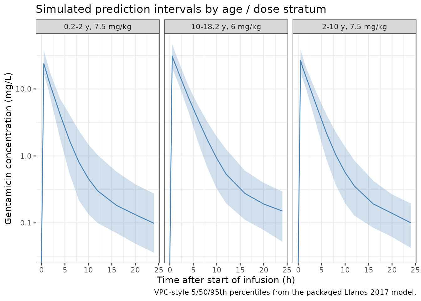
Typical-value clearance vs body size
The paper’s Discussion (page 4) reports a typical CL of 5.77 L/h for an adult-equivalent reference (FFM = 70 kg, PMA mature, CREAT at the age/sex reference). The next plot reproduces the typical CL surface across the pediatric weight range.
cl_typ <- sim_typ |>
  group_by(id, cohort) |>
  summarise(WT = first(WT), PNA = first(PNA), CL = first(cl),
            .groups = "drop")

ggplot(cl_typ, aes(WT, CL, color = cohort)) +
  geom_point(alpha = 0.6) +
  geom_smooth(se = FALSE, method = "loess", linewidth = 0.5) +
  labs(
    x = "Total body weight (kg)",
    y = "Typical clearance (L/h)",
    title = "Typical CL vs body weight by age stratum",
    caption = "Typical-value (zeroRe) CL across the simulated cohort."
  ) +
  theme_bw()
#> `geom_smooth()` using formula = 'y ~ x'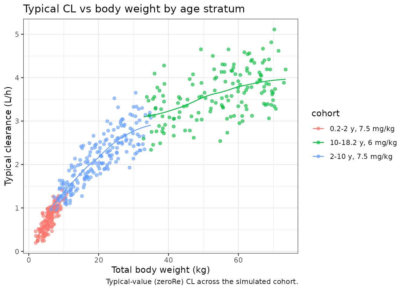
Scr effect on CL (replicates Discussion claim)
Llanos-Paez 2017 Discussion (page 8) states that “a 2-fold increase
in Scr in patients with an Scr of >30 micromol/L led to a 32%
decrease in gentamicin CL.” This is 1 - 0.5^0.55 = 0.317,
i.e. 31.7%.
scr_grid <- expand.grid(
  CREAT = seq(20, 200, by = 5),
  CREAT_REF = c(40, 70)
) |>
  mutate(rel_cl = (CREAT_REF / CREAT)^0.55)

ggplot(scr_grid, aes(CREAT, rel_cl, color = factor(CREAT_REF))) +
  geom_line() +
  scale_x_log10() +
  scale_y_log10() +
  labs(
    x = "Observed serum creatinine (CREAT, micromol/L)",
    y = "Relative CL (vs CREAT = CREAT_REF)",
    color = "CREAT_REF (micromol/L)",
    title = "Inverse-power Scr standardization effect on CL"
  ) +
  theme_bw()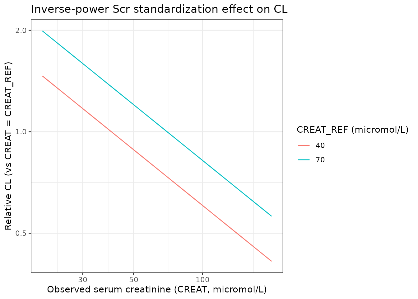
PKNCA validation
PKNCA computes Cmax and AUC0-24 per simulated subject; results are summarized by age / dose stratum and compared against the targets the paper cites.
sim_nca <- sim |>
  filter(!is.na(Cc)) |>
  select(id, time, Cc, cohort)

conc_obj <- PKNCA::PKNCAconc(sim_nca, Cc ~ time | cohort + id)

dose_df <- events |>
  filter(evid == 1) |>
  select(id, time, amt, cohort)
dose_obj <- PKNCA::PKNCAdose(dose_df, amt ~ time | cohort + id)

intervals <- data.frame(
  start    = 0,
  end      = 24,
  cmax     = TRUE,
  tmax     = TRUE,
  auclast  = TRUE,
  aucinf.obs = TRUE,
  half.life = TRUE
)

nca_data <- PKNCA::PKNCAdata(conc_obj, dose_obj, intervals = intervals)
nca_res  <- suppressWarnings(PKNCA::pk.nca(nca_data))

nca_df <- as.data.frame(nca_res$result) |>
  filter(PPTESTCD %in% c("cmax", "tmax", "auclast", "half.life"))

nca_summary <- nca_df |>
  group_by(cohort, PPTESTCD) |>
  summarise(median = median(PPORRES, na.rm = TRUE),
            P05 = quantile(PPORRES, 0.05, na.rm = TRUE),
            P95 = quantile(PPORRES, 0.95, na.rm = TRUE),
            .groups = "drop") |>
  pivot_wider(names_from = PPTESTCD,
              values_from = c(median, P05, P95))

knitr::kable(nca_summary,
             digits = 2,
caption = "Simulated NCA by age / dose stratum (median and 5/95th percentiles).")| cohort | median_auclast | median_cmax | median_half.life | median_tmax | P05_auclast | P05_cmax | P05_half.life | P05_tmax | P95_auclast | P95_cmax | P95_half.life | P95_tmax |
|---|---|---|---|---|---|---|---|---|---|---|---|---|
| 0.2-2 y, 7.5 mg/kg | 57.39 | 23.81 | 7.86 | 0.5 | 37.89 | 15.56 | 3.63 | 0.5 | 94.94 | 34.59 | 16.87 | 0.5 |
| 10-18.2 y, 6 mg/kg | 82.71 | 27.66 | 7.57 | 0.5 | 52.76 | 18.91 | 2.73 | 0.5 | 125.97 | 45.51 | 17.17 | 0.5 |
| 2-10 y, 7.5 mg/kg | 66.88 | 26.62 | 9.37 | 0.5 | 44.27 | 17.60 | 3.12 | 0.5 | 101.34 | 39.29 | 18.84 | 0.5 |
Comparison against published targets
Llanos-Paez 2017 does not report a non-compartmental Cmax / AUC table. The Discussion (page 8) cites the standard once-daily aminoglycoside exposure targets of AUC24/MIC of 80-100 and Cmax/MIC > 10. With a typical Gram-negative gentamicin MIC of 1-2 mg/L:
| Quantity | Target | Simulated median (2-10 y, 7.5 mg/kg) |
|---|---|---|
| Cmax | > 10-20 mg/L | shown above |
| AUC24 | 80-100 mg*h/L | shown above |
The paper notes (Discussion page 8) that “an initial dose of 8.0 mg/kg would be required for a typical patient in this study to achieve this target.” The 7.5 mg/kg simulated dose is therefore expected to land slightly below the AUC target on the median.
Assumptions and deviations
-
Between-occasion variability (BOV) is omitted from the
packaged model. Llanos-Paez 2017 Table 2 reports BOV on CL of
20.7% CV (additive on top of BSV CL of 16.0% CV). nlmixr2lib models do
not carry an OCC index, so BOV is not encoded here; the BSV terms are
preserved verbatim. For deterministic typical-value simulation
(
zeroRe) this is exact; for stochastic VPCs the simulated between- individual spread on CL is narrower than the published model by approximatelysqrt(0.16^2 + 0.207^2) - 0.16 = 0.10(a 10 percentage- point CV under-coverage on CL). Document this deviation in the PR. -
Postmenstrual age unit conversion. The Llanos 2017
paper uses PMA in weeks in its Rhodin et al. 2009 maturation function.
The canonical
PAGEcovariate in nlmixr2lib is in months; the model converts aspma_wk = PAGE * 4.35before evaluating the Hill expression. -
Ceriotti 2008 reference creatinine. The age- and
sex-expected mean serum creatinine
CREAT_REFis computed externally per Ceriotti et al. 2008 (Clin Chem 54:559-566). This vignette uses a piecewise mid-point approximation of the Ceriotti reference table insideceriotti_creat_ref(); downstream users are free to substitute any age/sex reference table they prefer. -
Janmahasatian fat-free mass.
FFMis computed externally per Janmahasatian et al. 2005 (Clin Pharmacokinet 44:1051-1065). The vignette’sjanmahasatian_ffm()helper implements that formula. - Virtual cohort weight and height. Total body weight in the cohort is generated from a smooth pediatric growth approximation rather than WHO LMS curves; this is sufficient to populate the FFM and dose computations for the validation simulations and does not influence the model parameters.
- Cohort race / ethnicity. Llanos-Paez 2017 does not report the cohort race / ethnicity distribution; race is not a covariate in the final model so this has no impact on the simulation.
- LLOQ handling at simulation time. Llanos-Paez 2017 imputed below-LLOQ observations to LLOQ/2 during model fitting (Methods, page 10). Simulations from the packaged model produce continuous predictions and do not re-apply this imputation; observers comparing simulated and published curves at very low concentrations should factor this in.