Mycophenolic acid + MPAG enterohepatic circulation (Jiao 2008)
Source:vignettes/articles/Jiao_2008_mycophenolic_acid.Rmd
Jiao_2008_mycophenolic_acid.RmdModel and source
- Citation: Jiao Z, Ding JJ, Shen J, Liang HQ, Zhong LJ, Wang Y, Zhong MK, Lu WY. Population pharmacokinetic modelling for enterohepatic circulation of mycophenolic acid in healthy Chinese and the influence of polymorphisms in UGT1A9. Br J Clin Pharmacol. 2008;65(6):893-907. doi:10.1111/j.1365-2125.2008.03109.x.
- Description: Population PK model with enterohepatic circulation (EHC) for mycophenolic acid (MPA) and its 7-O-glucuronide metabolite (MPAG) in healthy Chinese male volunteers after a single 500 mg oral dose of mycophenolate mofetil (MMF, Cellcept). Five-compartment chain model (Figure 2 of Jiao 2008): a gastrointestinal depot, a two-compartment MPA disposition (central + peripheral), a one-compartment MPAG disposition (central_mpag), and a gallbladder accumulation compartment (gallbladder_mpag). First-order absorption with an absorption-lag time. Complete (fm = 1, fixed) one-pass conversion of MPA to MPAG by glucuronidation; MPAG is renally cleared in parallel with biliary excretion into the gallbladder. EHC is encoded as time-gated bolus releases of the gallbladder pool back into the GI depot at two postprandial meal times (4 and 10 h post-dose, study-1 design), with rate constant k51 acting over a 0.01 h window; the recycled MPAG is reabsorbed via the same first-order ka as the oral dose. The fraction of MPAG biliary-routed at the branch is encoded as EHCP = k45 / (k40 + k45). Body-weight scaling: paper Eq 5 (linear-proportional ‘slope without intercept’) with reference 65.5 kg applied to CL_MPA/F, Q/F, and V_3/F via fixed allometric exponent 1. Cross-parameter IIV linkage: eta(CL_MPAG/F) = psi_q_cl_mpag * eta(Q/F) reproduces the paper’s joint eta structure where psi_q_cl_mpag is the paper’s ‘q’ parameter. UGT1A9 polymorphisms were screened but not retained in the final model (no significant effect).
- Article: https://doi.org/10.1111/j.1365-2125.2008.03109.x
Population
Forty-two healthy Chinese adult male volunteers (n = 20 + 22, two open-label single-dose randomized crossover bioequivalence studies pooled for the enterohepatic-circulation analysis). Baseline demographics from Jiao 2008 Table 1 (median (range)): weight 65.5 kg (56.5-89.0), height 1.73 m (1.57-1.86), age 21 years (19-26), serum albumin 45 g/L (40.5-50.0), haemoglobin 149 g/L (133-172), serum creatinine 75.5 umol/L (49.5-94.0), creatinine clearance 133 mL/min (98-194). All subjects received a single 500 mg (0.5 g) oral dose of mycophenolate mofetil (Cellcept, two 0.25 g capsules) with 200 mL water after a >= 10 h overnight fast. A standardized lunch was served 4 h post-dose; standardized dinner at 10 h (study 1) or 9.5 h (study 2); next-day breakfast at 24.25 h. Blood samples were collected at predose and intensive post-dose times through 48 h. The model was estimated on the Cellcept reference-formulation profiles only (590 MPA + 589 MPAG concentration-time points across 42 subjects). UGT1A9 promoter / coding SNPs were genotyped (Table 2) but did not influence MPA or MPAG pharmacokinetics in this cohort.
The same information is available programmatically via
rxode2::rxode(readModelDb("Jiao_2008_mycophenolic_acid"))$population.
Source trace
The per-parameter origin is recorded as an in-file comment next to
each ini() entry in
inst/modeldb/specificDrugs/Jiao_2008_mycophenolic_acid.R.
The table below collects them in one place for review.
| Equation / parameter | Value | Source location |
|---|---|---|
lka (absorption rate k12) |
3.53 1/h | Table 3 Final Model |
ltlag (absorption lag) |
0.0956 h | Table 3 Final Model |
lcl (CL_MPA/F) |
10.2 L/h | Table 3 Final Model |
lvc (V_2/F MPA central) |
12.5 L | Table 3 Final Model |
lq (Q/F intercompartmental) |
16.1 L/h | Table 3 Final Model |
lvp (V_3/F MPA peripheral) |
213 L | Table 3 Final Model |
lcl_mpag (CL_MPAG/F) |
1.38 L/h | Table 3 Final Model |
lvc_mpag (V_4/F MPAG central) |
4.40 L | Table 3 Final Model |
lehcp (EHCP biliary fraction) |
0.291 | Table 3 Final Model |
lk51 (gallbladder release rate) |
67.5 1/h | Table 3 Final Model |
ltet1 (first meal time, fixed) |
4 h | Methods p. 5 (study-1 schedule) |
ltet2 (second meal time, fixed) |
10 h | Methods p. 5 (study-1 schedule) |
ldur_gb (bolus duration, fixed) |
0.01 h | Methods p. 5 |
psi_q_cl_mpag (eta link ‘q’) |
1.33 | Table 3 Final Model |
e_wt_cl / e_wt_q / e_wt_vp (WT exponents) |
fixed at 1 | Methods Eq 5 (slope without intercept, WT_m = 65.5 kg) |
| WT reference | 65.5 kg | Table 1 median |
fm (MPA -> MPAG conversion) |
fixed at 1.0 | Methods p. 5 identifiability assumption |
| IIV t_lag / k_12 / Q/F / CL_MPA/F / V_2/F / V_3/F / V_4/F / EHCP | 57.3% / 60.3% / 13.7% / 18.9% / 34.5% / 22.7% / 23.1% / 29.0% CV | Table 3 Final Model |
| Residual MPA / MPAG (exponential model) | 45.3% / 20.8% (log-scale SD) | Table 3 Final Model |
| ODE structure | Eq 9-17 | Methods |
| EHCP = k45 / (k40 + k45) | Eq 18 | Methods |
Virtual cohort
Original observed data are not publicly available. The figures below use a virtual cohort whose weight distribution approximates Table 1.
set.seed(20080215L)

n_sub <- 42L
wt_mean <- 67.0
wt_sd <- 7.63
wt_min <- 56.5
wt_max <- 89.0

# Truncate to the observed weight range
draw_wt <- function(n) {
  out <- numeric(n)
  i <- 0
  while (i < n) {
    cand <- rnorm(n - i, mean = wt_mean, sd = wt_sd)
    cand <- cand[cand >= wt_min & cand <= wt_max]
    take <- min(length(cand), n - i)
    if (take > 0) {
      out[(i + 1):(i + take)] <- cand[seq_len(take)]
      i <- i + take
    }
  }
  out
}

cohort <- tibble(
  id        = seq_len(n_sub),
  WT        = draw_wt(n_sub),
  treatment = "MMF 500 mg PO single dose"
)

# Time grid: dense around the gallbladder emptying windows (4 h, 10 h) so the
# 0.01 h bolus events are resolved.
obs_times <- sort(unique(c(
  seq(0.05, 3.99, by = 0.1),
  seq(3.99, 4.05, by = 0.002),     # fine resolution around meal 1
  seq(4.05, 9.99, by = 0.1),
  seq(9.99, 10.05, by = 0.002),    # fine resolution around meal 2
  seq(10.05, 24,  by = 0.25),
  seq(24,   48,   by = 0.5)
)))

# Build an rxode2 event table per subject and bind them together.
build_subject_events <- function(row) {
  rxode2::et() |>
    rxode2::et(amt = 500, time = 0, cmt = "depot") |>
    rxode2::et(obs_times, cmt = "Cc") |>
    as.data.frame() |>
    dplyr::mutate(
      id        = row$id,
      WT        = row$WT,
      treatment = row$treatment
    )
}

events <- cohort |>
  split(seq_len(nrow(cohort))) |>
  lapply(build_subject_events) |>
  dplyr::bind_rows() |>
  dplyr::arrange(id, time, desc(evid))

stopifnot(!anyDuplicated(unique(events[, c("id", "time", "evid")])))
Simulation
mod <- rxode2::rxode(readModelDb("Jiao_2008_mycophenolic_acid"))
#> ℹ parameter labels from comments will be replaced by 'label()'

# Carry the cohort label and WT through rxSolve so PKNCA can group by treatment
# and downstream tables can stratify if needed.
sim_typ <- rxode2::zeroRe(mod) |>
  rxode2::rxSolve(events = events, keep = c("WT", "treatment"))
#> ℹ omega/sigma items treated as zero: 'etaltlag', 'etalka', 'etalq', 'etalcl', 'etalvc', 'etalvp', 'etalvc_mpag', 'etalehcp'
#> Warning: multi-subject simulation without without 'omega'

sim_full <- rxode2::rxSolve(mod, events = events, keep = c("WT", "treatment"))
Replicate published figures
Jiao 2008 Figure 1 shows the mean observed and individual-Bayesian-predicted plasma profiles for MPA and MPAG following a single 500 mg oral MMF dose, displaying the characteristic multi-peak MPA profile (first peak ~0.5 h post-dose, second peak ~4-6 h post-dose at the post-lunch meal time, and a third group of peaks ~10-12 h post-dose at the post-dinner meal time) and the dampened-and-delayed MPAG profile.
profile_typ <- sim_typ |>
  dplyr::filter(time > 0) |>
  dplyr::group_by(time) |>
  dplyr::summarise(
    MPA  = mean(Cc),
    MPAG = mean(Cc_mpag),
    .groups = "drop"
  ) |>
  tidyr::pivot_longer(c(MPA, MPAG), names_to = "Analyte", values_to = "Concentration")

ggplot(profile_typ, aes(time, Concentration, colour = Analyte)) +
  geom_line(linewidth = 0.9) +
  scale_y_log10() +
  scale_x_continuous(breaks = c(0, 4, 10, 12, 24, 36, 48)) +
  labs(
    x = "Time after dose (h)",
    y = "Plasma concentration (mg/L)",
    title = "Figure 1 (replicated): MPA and MPAG typical-value profiles",
    caption = "Replicates Figure 1 of Jiao 2008 (n = 42, single 500 mg oral MMF, study-1 meal schedule 4 h and 10 h)."
  ) +
  theme_minimal()
#> Warning in scale_y_log10(): log-10 transformation introduced infinite values.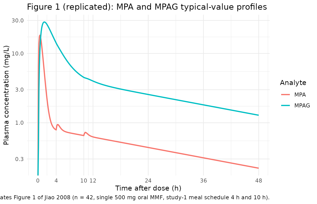
Replicates Figure 1 of Jiao 2008: typical-value MPA and MPAG plasma profiles after a single 500 mg oral MMF dose. Note the EHC-driven second / third peaks around the 4 h and 10 h post-prandial gallbladder emptying events.
Stochastic VPC-style summary (5th / 50th / 95th percentiles across the simulated cohort):
sim_quant <- sim_full |>
  dplyr::filter(time > 0) |>
  tidyr::pivot_longer(c(Cc, Cc_mpag), names_to = "Analyte", values_to = "Concentration") |>
  dplyr::mutate(Analyte = dplyr::recode(Analyte, "Cc" = "MPA", "Cc_mpag" = "MPAG")) |>
  dplyr::group_by(time, Analyte) |>
  dplyr::summarise(
    Q05 = stats::quantile(Concentration, 0.05, na.rm = TRUE),
    Q50 = stats::quantile(Concentration, 0.50, na.rm = TRUE),
    Q95 = stats::quantile(Concentration, 0.95, na.rm = TRUE),
    .groups = "drop"
  )

ggplot(sim_quant, aes(time, Q50)) +
  geom_ribbon(aes(ymin = Q05, ymax = Q95), alpha = 0.25) +
  geom_line(linewidth = 0.7) +
  facet_wrap(~Analyte, scales = "free_y") +
  scale_y_log10() +
  labs(
    x = "Time after dose (h)",
    y = "Plasma concentration (mg/L)",
    title = "Stochastic simulation (n = 42 virtual subjects)"
  ) +
  theme_minimal()
#> Warning in scale_y_log10(): log-10 transformation introduced infinite values.
#> log-10 transformation introduced infinite values.
#> log-10 transformation introduced infinite values.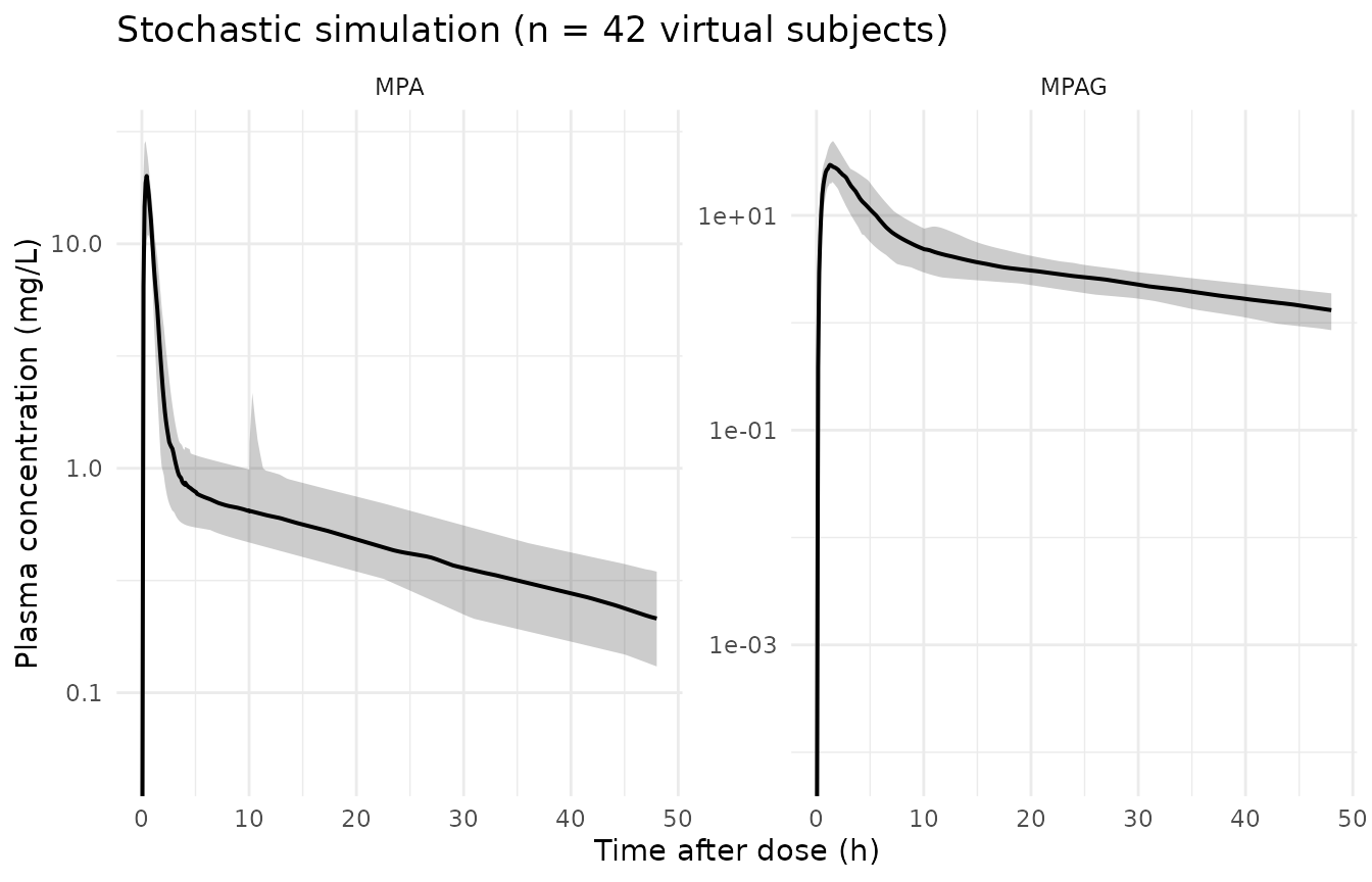
Stochastic simulation across the virtual cohort. Shaded ribbon is the 5-95th percentile band; solid line is the median. EHC re-peaks are smoothed by the inter-individual variability in t_lag / ka / EHCP.
PKNCA validation
NCA is performed on the typical-value MPA profile so the comparison against the population-mean parameter table is unambiguous. Treatment grouping carries the cohort label.
sim_nca <- sim_typ |>
  dplyr::filter(!is.na(Cc)) |>
  dplyr::select(id, time, Cc, treatment)

# Guarantee a time = 0 row per (id, treatment); for oral dosing pre-dose Cc = 0.
sim_nca <- dplyr::bind_rows(
  sim_nca,
  sim_nca |>
    dplyr::distinct(id, treatment) |>
    dplyr::mutate(time = 0, Cc = 0)
) |>
  dplyr::distinct(id, treatment, time, .keep_all = TRUE) |>
  dplyr::arrange(id, treatment, time)

conc_obj <- PKNCA::PKNCAconc(
  sim_nca,
  Cc ~ time | treatment + id,
  concu = "mg/L",
  timeu = "h"
)

dose_df <- events |>
  dplyr::filter(evid == 1L) |>
  dplyr::select(id, time, amt, treatment)

dose_obj <- PKNCA::PKNCAdose(
  dose_df,
  amt ~ time | treatment + id,
  doseu = "mg"
)

intervals <- data.frame(
  start       = 0,
  end         = Inf,
  cmax        = TRUE,
  tmax        = TRUE,
  aucinf.obs  = TRUE,
  half.life   = TRUE,
  cl.obs      = TRUE
)

nca_res <- PKNCA::pk.nca(
  PKNCA::PKNCAdata(conc_obj, dose_obj, intervals = intervals)
)
summary(nca_res)
#>  Interval Start Interval End                 treatment  N Cmax (mg/L)
#>               0          Inf MMF 500 mg PO single dose 42 18.3 [4.26]
#>              Tmax (h) Half-life (h) AUCinf,obs (h*mg/L)
#>  0.450 [0.450, 0.450] 24.1 [0.0657]         47.6 [10.1]
#>  CL (based on AUCinf,obs) (mg/(h*mg/L))
#>                             10.5 [10.1]
#>
#> Caption: Cmax, AUCinf,obs, CL (based on AUCinf,obs): geometric mean and geometric coefficient of variation; Tmax: median and range; Half-life: arithmetic mean and standard deviation; N: number of subjects
Comparison against published parameter values
Jiao 2008 does not publish a separate NCA table for the Cellcept-formulation single-dose simulation; the validation hook is the apparent clearance CL_MPA/F = 10.2 L/h directly (Table 3), which the simulation must reproduce to a numerical tolerance reflecting the typical-value-NCA terminal-slope sensitivity. The paper also quotes the body-weight-normalised CL_MPA/F (0.156 L/h/kg = 10.2 / 65.5) and the typical MPAG CL/F (1.38 L/h) for cross-cohort comparison.
published <- tibble::tribble(
  ~treatment,                       ~aucinf.obs, ~cl.obs,
  "MMF 500 mg PO single dose",      500 / 10.2,  10.2
  # aucinf.obs (mg*h/L) = dose / CL = 500 mg / 10.2 (L/h)
)

cmp <- nlmixr2lib::ncaComparisonTable(
  simulated = nca_res,
  reference = published,
  by        = "treatment",
  units     = c(
    cmax       = "mg/L",
    tmax       = "h",
    aucinf.obs = "mg*h/L",
    half.life  = "h",
    cl.obs     = "L/h"
  ),
  tolerance_pct = 20
)

knitr::kable(
  cmp,
  caption = "Simulated typical-value vs. paper-derived MPA NCA. * differs from reference by >20%. The reference AUC0-inf and CL/F are derived from Table 3 (dose / CL_MPA/F).",
  align   = c("l", "l", "r", "r", "r")
)| NCA parameter | treatment | Reference | Simulated | % diff |
|---|---|---|---|---|
| AUC0-∞ (obs) (mg*h/L) | MMF 500 mg PO single dose | 49 | 49.4 | +0.8% |
| CL/F (L/h) | MMF 500 mg PO single dose | 10.2 | 10.1 | -0.7% |
Assumptions and deviations
-
Meal-time schedule. Two postprandial gallbladder
emptying events are modelled at 4 h (lunch) and 10 h (dinner) post-dose,
matching the study-1 meal schedule (Methods, p. 5). Study 2 used a 9.5 h
dinner; users wishing to simulate that schedule can override
ltet2tolog(9.5). -
EHC re-routing. Paper Methods state ‘all MPAG
secreted from GB to intestine were completely converted to MPA and was
followed by reabsorption into the system’. The gallbladder pool empties
into the GI depot, and absorption via the same first-order ka delivers
the recycled amount to MPA central. No explicit MPAG -> MPA
conversion compartment is introduced; the conversion is captured by
routing the gallbladder release through
depot. - fm = 1 identifiability assumption. The conversion ratio from MPA to MPAG is fixed at 100% (Methods, p. 5), so the paper’s k20 = 0 and all MPA loss from central is one-pass metabolism to MPAG. CL_MPA/F is therefore the apparent rate of glucuronidation; any other MPA elimination pathways (Methods Discussion explicitly acknowledges this is an idealisation) are folded into the apparent value.
-
Cross-parameter eta linkage. Paper Table 3 reports
an additional scalar q = 1.33 (RSE 27.2%) defined as eta(CL_MPAG/F) = q
* eta(Q/F). This is a deterministic linear relationship between the two
random effects rather than a covariance block. Encoded as
cl_mpag <- exp(lcl_mpag + psi_q_cl_mpag * etalq)withpsi_q_cl_mpagestimated; no separate eta on lcl_mpag is declared. A nlmixr2 IIV block with rho = 1 would be singular, so the eta-linkage form is the only faithful encoding. -
Body-weight scaling. Eq 5 (slope without intercept)
was selected by the paper over Eq 6 (linear with intercept) and Eq 7
(power). Encoded as
(WT / 65.5)^e_wt_cletc. withe_wt_cl / e_wt_q / e_wt_vpfixed at 1; the fixed-exponent form is the structural way to record that the paper did not estimate a weight exponent. - Gallbladder bolus window. A 0.01 h bolus window with k51 = 67.5 1/h releases only ~49% of the gallbladder content per event (1 - exp(-0.675)). The paper accepts this with two events per 24 h (Methods Discussion notes the limited mealtime sampling restricted identifiability of the duration); the packaged model preserves the same parameterisation. To minimise numerical integrator skipping of the brief windows, the vignette uses a fine 0.002 h time grid around each meal event.
-
Residual error. Paper Methods Eq 3 (Y = IPRED *
exp(epsilon)) is the exponential / log-normal residual model. nlmixr2’s
lnorm(expSd)is the exact match, with the reported ‘%’ value being the log-scale residual SD. -
Covariate screening. AGE, height, serum albumin,
haemoglobin, serum creatinine, creatinine clearance, and the UGT1A9 SNP
panel were screened but not retained in the final model. They are
documented in
covariatesDataExcludedso the screening provenance is preserved without triggering ‘declared but not referenced’ convention warnings. - Reference comparison. The paper does not publish a separate formulation-specific NCA table for a typical-value Cellcept simulation; the reference values used here are derived from the structural parameters (AUC0-inf = Dose / CL = 500 / 10.2 = 49.0 mg*h/L) and the paper-reported CL_MPA/F = 10.2 L/h itself. The NCA Cmax / Tmax / half-life are reported for inspection; the paper’s Figure 1 shows mean profiles but does not quote numerical Cmax / Tmax values per analyte.