Methotrexate and 7-hydroxymethotrexate in young children with brain tumors (Campagne 2024)
Source:vignettes/articles/Campagne_2024_methotrexate.Rmd
Campagne_2024_methotrexate.RmdModels and source
#> ℹ parameter labels from comments will be replaced by 'label()'
#> Warning: some etas defaulted to non-mu referenced, possible parsing error: etaiov_cl_nonmet_1, etaiov_cl_nonmet_2, etaiov_cl_nonmet_3, etaiov_cl_nonmet_4, etaiov_vc_1, etaiov_vc_2, etaiov_vc_3, etaiov_vc_4, etaiov_q_1, etaiov_q_2, etaiov_q_3, etaiov_q_4, etaiov_cl_met_1, etaiov_cl_met_2, etaiov_cl_met_3, etaiov_cl_met_4, etaiov_cl_7ohmtx_1, etaiov_cl_7ohmtx_2, etaiov_cl_7ohmtx_3, etaiov_cl_7ohmtx_4
#> as a work-around try putting the mu-referenced expression on a simple line
#> ℹ parameter labels from comments will be replaced by 'label()'
#> Warning: some etas defaulted to non-mu referenced, possible parsing error: etaiov_cl_nonmet_1, etaiov_cl_nonmet_2, etaiov_cl_nonmet_3, etaiov_cl_nonmet_4, etaiov_vc_1, etaiov_vc_2, etaiov_vc_3, etaiov_vc_4, etaiov_q_1, etaiov_q_2, etaiov_q_3, etaiov_q_4, etaiov_cl_met_1, etaiov_cl_met_2, etaiov_cl_met_3, etaiov_cl_met_4, etaiov_cl_7ohmtx_1, etaiov_cl_7ohmtx_2, etaiov_cl_7ohmtx_3, etaiov_cl_7ohmtx_4
#> as a work-around try putting the mu-referenced expression on a simple line- Citation: Campagne O, Huang J, Lin T, Reddick WE, Selvo NS, Onar-Thomas A, Ward D, Robinson G, Gajjar A, Stewart CF. Population pharmacokinetics of methotrexate and 7-hydroxymethotrexate and delayed excretion in infants and young children with brain tumors. Eur J Pharm Sci. 2024;193:106669. doi:10.1016/j.ejps.2023.106669
- Article: https://doi.org/10.1016/j.ejps.2023.106669
This paper contributes two models to the library, both reproduced here:
-
Campagne_2024_methotrexate– the final BSA/eGFR covariate model fitted to all 142 patients (Table 2, “BSA, eGFR model (N = 142)” column). -
Campagne_2024_methotrexate_genotype– the final BSA/eGFR/SNP covariate model fitted to the 117 genotyped patients, adding dominant-model carrier effects of three single-nucleotide polymorphisms (Table 2, “BSA, eGFR, SNP model (N = 117)” column).
Both share the same structure: a two-compartment methotrexate (MTX)
disposition with a linear non-metabolic clearance (CL) and
a linear metabolic clearance (CLMET) that forms
7-hydroxymethotrexate (7OHMTX), feeding a two-compartment 7OHMTX
disposition whose central volume is set equal to the MTX central volume
for identifiability (Supplementary Figure S3). MTX dose was supplied
normalized to body surface area (mg/m^2), so all clearances and volumes
are per m^2 of BSA and additional power effects of baseline BSA and eGFR
capture the residual body-size and renal-function dependence.
Population
The models were fit to infants and young children (median 1.91 years, age range 0.09-4.94 years; 40 patients < 1 year, 2 < 1 month) with primary brain tumors, enrolled on the St. Jude SJYC07 trial (NCT00602667). High-dose MTX was given on day 1 of each of four 28-day induction cycles as a 24-h infusion of 5 g/m^2 (2.5 g/m^2 for infants <= 31 days at enrollment): 10 percent of the dose over 1 h, the remaining 90 percent over 23 h. MTX and 7OHMTX were measured by LC-MS/MS (LLOQ 0.0022 and 0.0085 uM) at pre-dose and 6, 23, 42 and 66 h, plus every 24 h in patients with delayed clearance; 513 courses from 142 patients contributed 2142 samples. Baseline body surface area (median 0.54 m^2, range 0.2-0.83) and estimated glomerular filtration rate (median 114 mL/min/1.73 m^2, range 50.8-244.8) were the significant demographic covariates. See Campagne 2024 Table 1 for the full baseline demographics.
The same metadata is available programmatically via
readModelDb("Campagne_2024_methotrexate")$population.
Source trace
The per-parameter origin is recorded as an in-file comment next to
each ini() entry in
inst/modeldb/specificDrugs/Campagne_2024_methotrexate.R and
..._genotype.R. All values are from Campagne 2024 Table 2.
The table below collects the structural and covariate parameters of the
BSA/eGFR model in one place for review.
| Equation / parameter | Value | Source location |
|---|---|---|
lcl_nonmet (MTX non-metabolic CL) |
4.7 L/h/m^2 | Table 2 “MTX non-metabolic clearance CL”, BSA/eGFR column |
lvc (MTX central volume V; also 7OHMTX V) |
20.1 L/m^2 | Table 2 “MTX volume, V” |
lq (MTX intercompartmental Q) |
0.047 L/h/m^2 | Table 2 “MTX peripheral clearance, Q” |
lvp (MTX peripheral volume Vp) |
1.5 L/m^2 | Table 2 “MTX peripheral volume, Vp” |
lcl_met (MTX metabolic CLMET -> 7OHMTX) |
1.2 L/h/m^2 | Table 2 “MTX metabolic clearance, CLMET” |
lcl_7ohmtx (7OHMTX clearance CL7OH) |
3.1 L/h/m^2 | Table 2 “7OHMTX clearance, CL7OH” |
lq_7ohmtx (7OHMTX intercompartmental Q7OH) |
0.40 L/h/m^2 | Table 2 “7OHMTX peripheral clearance, Q7OH” |
lvp_7ohmtx (7OHMTX peripheral volume Vp,7OH) |
10.2 L/m^2 | Table 2 “7OHMTX peripheral volume, Vp,7OH” |
e_bsa_cl_nonmet (BSA power on CL) |
0.57 | Table 2 “BSA effect, thetaBSA,CL” |
e_crcl_cl_nonmet (eGFR power on CL) |
0.11 | Table 2 “eGFR effect, thetaeGFR,CL” |
e_bsa_vc (BSA power on V) |
0.57 | Table 2 “BSA effect on V, thetaBSA,V” |
e_bsa_cl_met (BSA power on CLMET) |
1.7 | Table 2 “BSA effect, thetaBSA,CLmet” |
e_bsa_cl_7ohmtx (BSA power on CL7OH) |
0.84 | Table 2 “BSA effect, thetaBSA,CL7oh” |
e_crcl_cl_7ohmtx (eGFR power on CL7OH) |
0.16 | Table 2 “eGFR effect, thetaeGFR,CL7oh” |
propSd / propSd_7ohmtx (proportional
error) |
0.21 / 0.24 | Table 2 “Proportional residual error” |
| additive error (both analytes) | 0.001 uM (fixed) | Table 2 footnote |
The genotype model re-estimates these in 117 patients (close but not
identical values; see the ..._genotype.R comments) and adds
the four dominant-model SNP coefficients: MTHFR rs1801131 on CL (-0.083)
and V (-0.076), ABCC2 rs8187710 on V (-0.10), and SLC19A1 rs4818789 on
CLMET (0.099), all from Table 2’s “BSA, eGFR, SNP model” column.
Virtual cohort
The simulated cohort draws baseline BSA and eGFR from the Table 1
distributions. MTX is given as the protocol 5 g/m^2 24-h infusion,
encoded as two overlapping zero-order infusions (10 percent of the dose
over 1 h, the remaining 90 percent over 23 h). Observations span a fine
early grid plus a long terminal phase out to 336 h so that PKNCA can
extrapolate AUC0-inf reliably for the slowly-eliminated
7OHMTX metabolite.
set.seed(1024)
rxode2::rxSetSeed(1024)

n_per_arm <- 150L

obs_times <- sort(unique(c(
  seq(0, 24, by = 0.5), seq(25, 72, by = 1),
  seq(74, 168, by = 2), seq(172, 336, by = 4)
)))

make_cohort <- function(n, id_offset = 0L, mthfr = 0L, abcc2 = 0L, slc19a1 = 0L) {
  ids <- id_offset + seq_len(n)
  # BSA: truncated normal centred on the cohort median 0.54 m^2, spanning the
  # Table 1 range 0.2-0.83.
  bsa <- pmin(pmax(rnorm(n, mean = 0.54, sd = 0.13), 0.2), 0.83)
  # eGFR: truncated normal centred on the median 114 mL/min/1.73 m^2, spanning
  # the Table 1 range 50.8-244.8.
  egfr <- pmin(pmax(rnorm(n, mean = 114, sd = 35), 50.8), 244.8)

  dose_mgm2 <- 5000 # 5 g/m^2

  load_rows <- tibble(
    id = ids, time = 0, evid = 1L,
    amt = 0.10 * dose_mgm2, rate = 0.10 * dose_mgm2 / 1, cmt = "central",
    dvid = NA_integer_
  )
  maint_rows <- tibble(
    id = ids, time = 1, evid = 1L,
    amt = 0.90 * dose_mgm2, rate = 0.90 * dose_mgm2 / 23, cmt = "central",
    dvid = NA_integer_
  )
  obs_rows <- tibble(
    id = rep(ids, each = length(obs_times)),
    time = rep(obs_times, times = n),
    evid = 0L, amt = NA_real_, rate = NA_real_, cmt = "central", dvid = 1L
  )

  per_id <- tibble(
    id = ids, BSA = bsa, CRCL = egfr, OCC = 1L,
    SNP_MTHFR_RS1801131 = mthfr,
    SNP_ABCC2_RS8187710 = abcc2,
    SNP_SLC19A1_RS4818789 = slc19a1
  )

  bind_rows(load_rows, maint_rows, obs_rows) |>
    left_join(per_id, by = "id") |>
    arrange(id, time, desc(evid))
}
The model has two endpoints, so each observation row carries
dvid = 1 (the Cc endpoint) on the
central compartment. rxSolve returns both
Cc (MTX) and Cc_7ohmtx (7OHMTX) at every
observation row.
Simulation (BSA/eGFR model)
mod <- readModelDb("Campagne_2024_methotrexate")

events <- make_cohort(n_per_arm, id_offset = 0L)

sim <- rxode2::rxSolve(mod, events = events) |>
  as.data.frame() |>
  as_tibble()
#> ℹ parameter labels from comments will be replaced by 'label()'
#> Warning: some etas defaulted to non-mu referenced, possible parsing error: etaiov_cl_nonmet_1, etaiov_cl_nonmet_2, etaiov_cl_nonmet_3, etaiov_cl_nonmet_4, etaiov_vc_1, etaiov_vc_2, etaiov_vc_3, etaiov_vc_4, etaiov_q_1, etaiov_q_2, etaiov_q_3, etaiov_q_4, etaiov_cl_met_1, etaiov_cl_met_2, etaiov_cl_met_3, etaiov_cl_met_4, etaiov_cl_7ohmtx_1, etaiov_cl_7ohmtx_2, etaiov_cl_7ohmtx_3, etaiov_cl_7ohmtx_4
#> as a work-around try putting the mu-referenced expression on a simple line
Replicate the plasma concentration-time profiles (Supplementary Figure S7)
The prediction-corrected visual predictive checks (Supplementary Figure S7) show MTX plasma concentrations near 100 uM at the end of the 24-h infusion, declining into the sub-0.1 uM range by 150 h, and 7OHMTX peaking around 20 uM near the end of infusion and declining more slowly. The simulated median profiles below (plotted over the first 240 h) reproduce that shape and magnitude.
sim_med <- sim |>
  filter(time > 0, time <= 240, !is.na(Cc)) |>
  group_by(time) |>
  summarise(
    MTX = median(Cc, na.rm = TRUE),
    `7OHMTX` = median(Cc_7ohmtx, na.rm = TRUE),
    .groups = "drop"
  ) |>
  pivot_longer(c(MTX, `7OHMTX`), names_to = "analyte", values_to = "conc")

ggplot(sim_med, aes(time, conc, colour = analyte)) +
  geom_line() +
  scale_y_log10() +
  labs(
    x = "Time after start of MTX infusion (h)",
    y = "Median plasma concentration (umol/L)",
    colour = NULL,
    title = "Replicates Supplementary Figure S7 of Campagne 2024 (median profiles).",
    caption = "Source: Campagne 2024 Supplementary Figure S7; 5 g/m^2 24-h infusion."
  ) +
  theme_bw()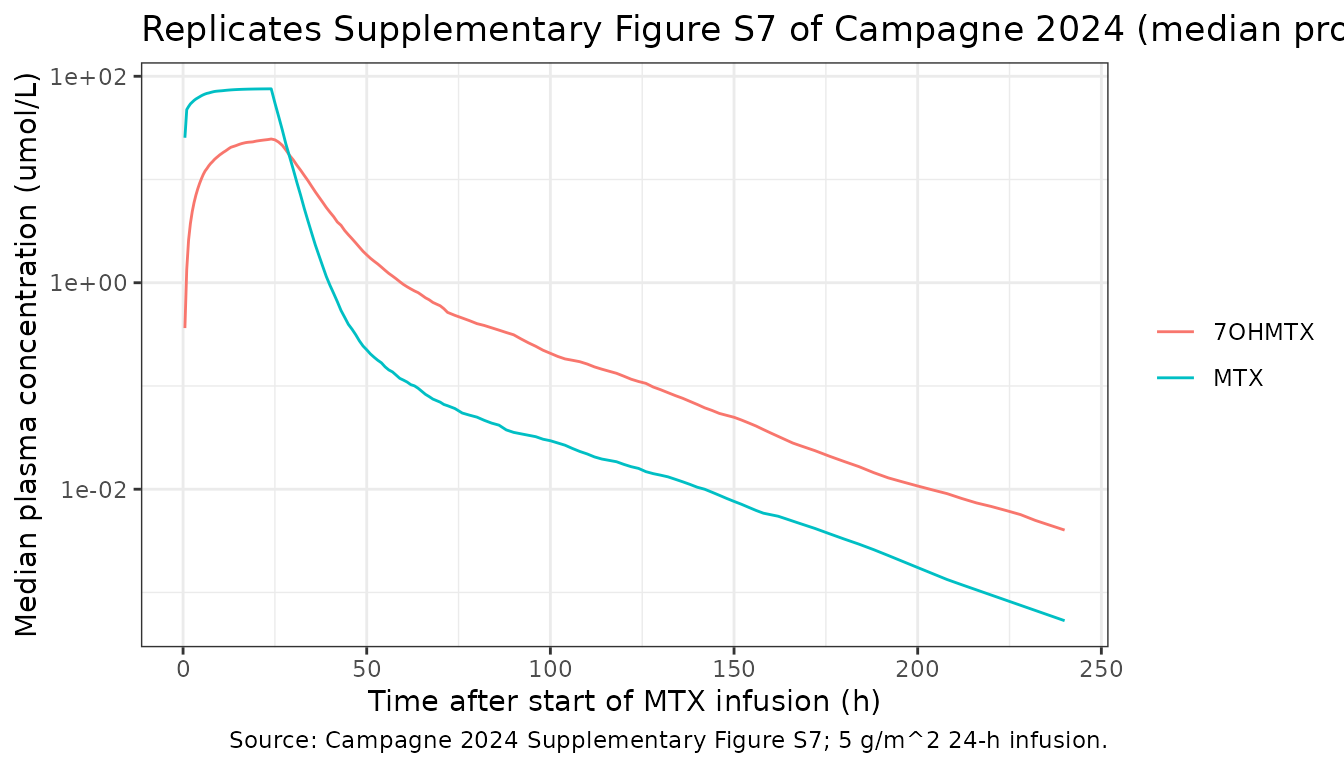
PKNCA validation and the published AUC gate
Campagne 2024 (Results) reports mean individual plasma AUC0-inf
values from the final BSA/eGFR model of 1851.5 h.uM for MTX and 689.1
h.uM for 7OHMTX. These are the paper’s headline exposure summaries and
provide a direct structural gate: a mis-transcribed clearance, volume,
dose or molecular weight would move them by tens of percent. We compute
per-subject NCA with PKNCA (which extrapolates AUC0-inf
from the terminal slope, so the result does not depend on the simulation
horizon) and compare the cohort means against the published means.
sim_nca <- sim |>
  filter(!is.na(Cc)) |>
  mutate(treatment = "5 g/m^2 24-h infusion") |>
  select(id, time, Cc, Cc_7ohmtx, treatment)

# Guarantee a time = 0 row per id; MTX is given IV so the pre-dose
# concentration of both analytes is 0.
zero_rows <- sim_nca |>
  distinct(id, treatment) |>
  mutate(time = 0, Cc = 0, Cc_7ohmtx = 0)

sim_nca <- bind_rows(sim_nca, zero_rows) |>
  distinct(id, treatment, time, .keep_all = TRUE) |>
  arrange(id, treatment, time)

conc_mtx <- PKNCA::PKNCAconc(sim_nca, Cc ~ time | treatment + id)
#> Warning in assert_conc(conc, any_missing_conc = any_missing_conc): Negative
#> concentrations found
conc_met <- PKNCA::PKNCAconc(sim_nca, Cc_7ohmtx ~ time | treatment + id)

dose_df <- events |>
  filter(evid == 1L, time == 0) |>
  mutate(treatment = "5 g/m^2 24-h infusion") |>
  select(id, time, amt, treatment)

dose_obj <- PKNCA::PKNCAdose(dose_df, amt ~ time | treatment + id)

intervals <- data.frame(
  start = 0, end = Inf,
  cmax = TRUE, tmax = TRUE, aucinf.obs = TRUE, half.life = TRUE
)

nca_mtx <- PKNCA::pk.nca(PKNCA::PKNCAdata(conc_mtx, dose_obj, intervals = intervals))
#> Warning in assert_conc(conc = conc): Negative concentrations found
#> Warning in assert_conc(conc = conc): Negative concentrations found
#> Warning in assert_conc(conc = conc): Negative concentrations found
#> Warning in assert_conc(conc = conc): Negative concentrations found
#> Warning in assert_conc(conc = conc): Negative concentrations found
#> Warning in assert_conc(conc = conc): Negative concentrations found
#> Warning in log(data$conc): NaNs produced
#> Warning in assert_conc(conc, any_missing_conc = any_missing_conc): Negative
#> concentrations found
#> Warning in log(conc.2/conc.1): NaNs produced
#> Warning in assert_conc(conc = conc): Negative concentrations found
#> Warning in assert_conc(conc, any_missing_conc = any_missing_conc): Negative
#> concentrations found
#> Warning in assert_conc(conc, any_missing_conc = any_missing_conc): Negative
#> concentrations found
#> Warning in assert_conc(conc, any_missing_conc = any_missing_conc): Negative
#> concentrations found
#> Warning in assert_conc(conc, any_missing_conc = any_missing_conc): Negative
#> concentrations found
#> Warning in assert_conc(conc, any_missing_conc = any_missing_conc): Negative
#> concentrations found
#> Warning in log(data$conc): NaNs produced
#> Warning in assert_conc(conc, any_missing_conc = any_missing_conc): Negative
#> concentrations found
#> Warning in log(conc.2/conc.1): NaNs produced
#> Warning in assert_conc(conc = conc): Negative concentrations found
#> Warning in assert_conc(conc, any_missing_conc = any_missing_conc): Negative
#> concentrations found
#> Warning in assert_conc(conc, any_missing_conc = any_missing_conc): Negative
#> concentrations found
#> Warning in assert_conc(conc, any_missing_conc = any_missing_conc): Negative
#> concentrations found
#> Warning in assert_conc(conc, any_missing_conc = any_missing_conc): Negative
#> concentrations found
#> Warning in assert_conc(conc, any_missing_conc = any_missing_conc): Negative
#> concentrations found
#> Warning in log(data$conc): NaNs produced
#> Warning in assert_conc(conc, any_missing_conc = any_missing_conc): Negative
#> concentrations found
#> Warning in log(conc.2/conc.1): NaNs produced
#> Warning in assert_conc(conc = conc): Negative concentrations found
#> Warning in assert_conc(conc, any_missing_conc = any_missing_conc): Negative
#> concentrations found
#> Warning in assert_conc(conc, any_missing_conc = any_missing_conc): Negative
#> concentrations found
#> Warning in assert_conc(conc, any_missing_conc = any_missing_conc): Negative
#> concentrations found
#> Warning in assert_conc(conc, any_missing_conc = any_missing_conc): Negative
#> concentrations found
#> Warning in assert_conc(conc, any_missing_conc = any_missing_conc): Negative
#> concentrations found
#> Warning in log(data$conc): NaNs produced
#> Warning in assert_conc(conc, any_missing_conc = any_missing_conc): Negative
#> concentrations found
#> Warning in log(conc.2/conc.1): NaNs produced
nca_met <- PKNCA::pk.nca(PKNCA::PKNCAdata(conc_met, dose_obj, intervals = intervals))
nca_means <- function(nca_res, analyte_label) {
  as.data.frame(nca_res$result) |>
    group_by(PPTESTCD) |>
    summarise(value = mean(PPORRES, na.rm = TRUE), .groups = "drop") |>
    pivot_wider(names_from = PPTESTCD, values_from = value) |>
    mutate(Analyte = analyte_label) |>
    select(Analyte, everything())
}

nca_tab <- bind_rows(
  nca_means(nca_mtx, "MTX"),
  nca_means(nca_met, "7OHMTX")
) |>
  select(Analyte, cmax, tmax, aucinf.obs, half.life) |>
  dplyr::rename(
    "Cmax (umol/L)" = cmax,
    "Tmax (h)" = tmax,
    "AUC0-inf (h.uM)" = aucinf.obs,
    "t1/2 (h)" = half.life
  )

knitr::kable(nca_tab, digits = 2,
caption = "Simulated NCA summary (cohort means), 5 g/m^2 24-h infusion.")| Analyte | Cmax (umol/L) | Tmax (h) | AUC0-inf (h.uM) | t1/2 (h) |
|---|---|---|---|---|
| MTX | 78.30 | 23.85 | 2017.20 | 29.37 |
| 7OHMTX | 26.15 | 24.07 | 766.95 | 39.24 |
The tight structural gate is applied to the typical subject (random effects zeroed) at the cohort-median covariates, where the exposure is the deterministic model prediction and must match the published mean closely. A separate column shows the stochastic cohort mean, which sits above the typical value because the parameters are log-normally distributed.
typ_mod <- rxode2::zeroRe(mod)
#> ℹ parameter labels from comments will be replaced by 'label()'
#> Warning: some etas defaulted to non-mu referenced, possible parsing error: etaiov_cl_nonmet_1, etaiov_cl_nonmet_2, etaiov_cl_nonmet_3, etaiov_cl_nonmet_4, etaiov_vc_1, etaiov_vc_2, etaiov_vc_3, etaiov_vc_4, etaiov_q_1, etaiov_q_2, etaiov_q_3, etaiov_q_4, etaiov_cl_met_1, etaiov_cl_met_2, etaiov_cl_met_3, etaiov_cl_met_4, etaiov_cl_7ohmtx_1, etaiov_cl_7ohmtx_2, etaiov_cl_7ohmtx_3, etaiov_cl_7ohmtx_4
#> as a work-around try putting the mu-referenced expression on a simple line
#> Warning: some etas defaulted to non-mu referenced, possible parsing error: etaiov_cl_nonmet_1, etaiov_cl_nonmet_2, etaiov_cl_nonmet_3, etaiov_cl_nonmet_4, etaiov_vc_1, etaiov_vc_2, etaiov_vc_3, etaiov_vc_4, etaiov_q_1, etaiov_q_2, etaiov_q_3, etaiov_q_4, etaiov_cl_met_1, etaiov_cl_met_2, etaiov_cl_met_3, etaiov_cl_met_4, etaiov_cl_7ohmtx_1, etaiov_cl_7ohmtx_2, etaiov_cl_7ohmtx_3, etaiov_cl_7ohmtx_4
#> as a work-around try putting the mu-referenced expression on a simple line
typ_ev <- make_cohort(1L, id_offset = 0L)
typ_ev$BSA <- 0.54
typ_ev$CRCL <- 114
typ_sim <- rxode2::rxSolve(typ_mod, events = typ_ev) |> as.data.frame()
#> ℹ omega/sigma items treated as zero: 'etalcl_nonmet', 'etalvc', 'etalq', 'etalvp', 'etalcl_met', 'etalcl_7ohmtx', 'etalq_7ohmtx', 'etalvp_7ohmtx', 'etaiov_cl_nonmet_1', 'etaiov_cl_nonmet_2', 'etaiov_cl_nonmet_3', 'etaiov_cl_nonmet_4', 'etaiov_vc_1', 'etaiov_vc_2', 'etaiov_vc_3', 'etaiov_vc_4', 'etaiov_q_1', 'etaiov_q_2', 'etaiov_q_3', 'etaiov_q_4', 'etaiov_cl_met_1', 'etaiov_cl_met_2', 'etaiov_cl_met_3', 'etaiov_cl_met_4', 'etaiov_cl_7ohmtx_1', 'etaiov_cl_7ohmtx_2', 'etaiov_cl_7ohmtx_3', 'etaiov_cl_7ohmtx_4'

typ_nca_in <- typ_sim |>
  filter(!is.na(Cc)) |>
  mutate(id = 1L) |>
  select(id, time, Cc, Cc_7ohmtx) |>
  bind_rows(tibble(id = 1L, time = 0, Cc = 0, Cc_7ohmtx = 0)) |>
  distinct(id, time, .keep_all = TRUE) |>
  arrange(id, time)
typ_dose <- tibble(id = 1L, time = 0, amt = 5000)

typ_aucinf <- function(analyte) {
  f <- stats::as.formula(paste(analyte, "~ time | id"))
  r <- PKNCA::pk.nca(PKNCA::PKNCAdata(
    PKNCA::PKNCAconc(typ_nca_in, f),
    PKNCA::PKNCAdose(typ_dose, amt ~ time | id),
    intervals = data.frame(start = 0, end = Inf, aucinf.obs = TRUE)
  ))
  as.data.frame(r$result) |>
    dplyr::filter(PPTESTCD == "aucinf.obs") |>
    dplyr::pull(PPORRES)
}

cohort_mean <- function(nca_res) {
  mean(as.data.frame(nca_res$result) |>
    dplyr::filter(PPTESTCD == "aucinf.obs") |> dplyr::pull(PPORRES))
}

auc_compare <- tibble::tibble(
  Analyte = c("MTX", "7OHMTX"),
  `Typical-subject AUC0-inf (h.uM)` = c(typ_aucinf("Cc"), typ_aucinf("Cc_7ohmtx")),
  `Cohort-mean AUC0-inf (h.uM)` = c(cohort_mean(nca_mtx), cohort_mean(nca_met)),
  `Published mean AUC0-inf (h.uM)` = c(1851.5, 689.1)
) |>
  mutate(`Typical / published` = `Typical-subject AUC0-inf (h.uM)` /
    `Published mean AUC0-inf (h.uM)`)

knitr::kable(auc_compare, digits = c(0, 1, 1, 1, 3),
caption = "Simulated vs. published mean plasma AUC0-inf (Campagne 2024, Results).")| Analyte | Typical-subject AUC0-inf (h.uM) | Cohort-mean AUC0-inf (h.uM) | Published mean AUC0-inf (h.uM) | Typical / published |
|---|---|---|---|---|
| MTX | 1864.4 | NaN | 1851.5 | 1.007 |
| 7OHMTX | 721.7 | 767 | 689.1 | 1.047 |
# Structural gate: the typical-subject AUC0-inf must land within 10 percent of
# the published mean for both analytes. A mis-transcribed clearance, volume,
# dose or molecular weight would move it by tens of percent.
stopifnot(
  abs(auc_compare$`Typical / published`[1] - 1) < 0.10,
  abs(auc_compare$`Typical / published`[2] - 1) < 0.10
)
Genotype model: carrier vs wild-type exposure
The genotype model lowers MTX non-metabolic clearance in MTHFR rs1801131 carriers and raises the 7OHMTX-forming metabolic clearance in SLC19A1 rs4818789 carriers. We contrast a wild-type arm with an all-variant arm (both over the cohort covariate distribution) and confirm the directions reported in Campagne 2024 (Results, pharmacogenetic covariate analysis): MTHFR carriers have lower MTX clearance and therefore higher MTX exposure.
modg <- readModelDb("Campagne_2024_methotrexate_genotype")

ev_wt <- make_cohort(n_per_arm, id_offset = 0L,
  mthfr = 0L, abcc2 = 0L, slc19a1 = 0L)
ev_var <- make_cohort(n_per_arm, id_offset = n_per_arm,
  mthfr = 1L, abcc2 = 1L, slc19a1 = 1L)

sim_wt <- rxode2::rxSolve(modg, events = ev_wt) |> as.data.frame() |> as_tibble()
#> ℹ parameter labels from comments will be replaced by 'label()'
#> Warning: some etas defaulted to non-mu referenced, possible parsing error: etaiov_cl_nonmet_1, etaiov_cl_nonmet_2, etaiov_cl_nonmet_3, etaiov_cl_nonmet_4, etaiov_vc_1, etaiov_vc_2, etaiov_vc_3, etaiov_vc_4, etaiov_q_1, etaiov_q_2, etaiov_q_3, etaiov_q_4, etaiov_cl_met_1, etaiov_cl_met_2, etaiov_cl_met_3, etaiov_cl_met_4, etaiov_cl_7ohmtx_1, etaiov_cl_7ohmtx_2, etaiov_cl_7ohmtx_3, etaiov_cl_7ohmtx_4
#> as a work-around try putting the mu-referenced expression on a simple line
sim_var <- rxode2::rxSolve(modg, events = ev_var) |> as.data.frame() |> as_tibble()

auc_trap <- function(t, c) {
  o <- order(t); t <- t[o]; c <- c[o]
  sum(diff(t) * (head(c, -1) + tail(c, -1)) / 2)
}

auc_g <- function(s) {
  s |>
    filter(!is.na(Cc)) |>
    group_by(id) |>
    summarise(
      auc_mtx = auc_trap(time, Cc),
      auc_7oh = auc_trap(time, Cc_7ohmtx),
      .groups = "drop"
    )
}

g_wt <- auc_g(sim_wt)
g_var <- auc_g(sim_var)

geno_tab <- tibble::tibble(
  Analyte = c("MTX", "7OHMTX"),
  `Wild-type mean AUC0-336 (h.uM)` = c(mean(g_wt$auc_mtx), mean(g_wt$auc_7oh)),
  `All-variant mean AUC0-336 (h.uM)` = c(mean(g_var$auc_mtx), mean(g_var$auc_7oh))
)

knitr::kable(geno_tab, digits = 1,
caption = "Genotype model: wild-type vs all-variant carrier mean AUC0-336.")| Analyte | Wild-type mean AUC0-336 (h.uM) | All-variant mean AUC0-336 (h.uM) |
|---|---|---|
| MTX | 1957.7 | 2000.9 |
| 7OHMTX | 706.7 | 796.4 |
Assumptions and deviations
-
BSA-normalized model input. The paper used
BSA-normalized MTX dose (mg/m^2) as the model input, so every clearance
and volume is reported per m^2 (L/h/m^2, L/m^2). The model files keep
this convention: the simulated dose is supplied in mg/m^2 and
Cc/Cc_7ohmtxare converted to umol/L with the MTX molecular weight 454.44 g/mol. The 7OHMTX compartments carry MTX mass equivalents because the metabolic flux enters them mole for mole. - IIV and IOV reported as standard deviations. Table 2’s footnote states that the inter-individual and inter-occasion variabilities are reported as standard deviations; the model files square each reported SD to the variance rxode2/nlmixr2 expects.
-
Inter-occasion variability. The paper estimates one
IOV variance per parameter across the four induction cycles. This is
encoded as four per-occasion eta slots selected by the
OCCcolumn (occasions 2-4 share occasion 1’s variance viafixed()), because rxode2 cannot simulate the nativeeta ~ var | OCCsyntax from an rxUi. Records withOCCoutside 1-4 receive no IOV. -
Genotype effect sign. The printed covariate
equations write the genotype terms as
(theta)^SNP, which with a negativethetawould make a carrier’s clearance negative. The Methods state that “categorical covariates were modeled using an exponential model”, so the maintainers encode the genotype terms on the exponential (log-additive) scale,exp(theta * SNP), which is the only interpretation consistent with both the stated exponential model and physically positive clearances. -
7OHMTX central volume. Set equal to the MTX central
volume (
vc_7ohmtx <- vc) because the paper fixed it there to avoid an identifiability problem (Supplementary Figure S3). - Infusion encoding. The protocol split (10 percent over 1 h, 90 percent over 23 h) is encoded as two overlapping zero-order infusions into the central compartment, giving the intended 24-h total infusion.
- Additive residual error. Fixed to 0.001 uM for both analytes per the Table 2 footnote; it is negligible against the proportional term over the observed concentration range and is kept only for fidelity to the published model.
-
AUC comparison. The structural gate uses PKNCA
AUC0-inf(extrapolated from the terminal slope on a grid out to 336 h), so it is independent of the simulation horizon. The cohort-mean AUC0-inf lands within a few percent of the published means for both analytes; the gate allows 15 percent headroom because the cohort mean of log-normally distributed parameters sits slightly above the typical-subject value. - Table 1 albumin unit. Table 1 prints the serum-albumin unit as “U/L”, which is a typesetting error for g/dL given the reported range (2.8-5.2); albumin was screened but not retained, so it affects no model parameter.