Trazodone + gabapentin writhing PK/PD in mice and human translation (Oggianu 2023)
Source:vignettes/articles/Oggianu_2023_trazodone_gabapentin.Rmd
Oggianu_2023_trazodone_gabapentin.RmdModel and source
- Citation: Oggianu L, Ottaviani M, Maddalena F, et al. PK/PD analysis of trazodone and gabapentin in neuropathic pain rodent models: Translational PK-PD modeling from nonclinical to clinical development. Clin Transl Sci 2023;16(4):606-617. doi:10.1111/cts.13472 (open access via PMC10087074).
- Models:
-
Oggianu_2023_trazodone_gabapentin_mouse– Preclinical (mouse, male CD-1). Joint PK/PD model of the antinociceptive interaction of oral trazodone and intraperitoneal gabapentin in the acetic-acid writhing test. Each drug has zero-order input and two-compartment disposition parameterised by micro-constants. The intraperitoneal acetic-acid stimulus is a unit dose into a stimulus compartment scaled by the stimulus amplitude S; it passes through nine transit compartments into the observed writhing compartment, which empties first-order. Each drug removes stimulus in proportion to its plasma molar concentration, and a product term on the two concentrations carries the departure from additivity (synergy). Time is in minutes; the PK parameters keep their published hour units and are converted in model(). -
Oggianu_2023_trazodone_human– Two-compartment population PK model of oral trazodone (immediate-release tablet and 6% oral drops) with first-order absorption and a lag time in healthy adult volunteers, carrying the authors’ translational writhing layer: the human plasma concentration, rescaled to the mouse unbound fraction, drives the mouse acetic-acid writhing PD model (stimulus, nine transit compartments, writhing compartment) with the mouse trazodone potency, as used to predict the percent inhibition of a pain stimulus at low human doses. The writhing layer is a cross-species projection, not a fit to human PD data.
-
Angelini developed a low-dose fixed combination of trazodone and gabapentin for neuropathic pain. Oggianu and colleagues quantified the interaction of the two drugs in the mouse acetic-acid writhing test with a sequential PK/PD analysis, then projected the mouse PD onto human trazodone exposure to suggest clinical starting doses.
The writhing model (Supplementary Table S1 and Figure S1) treats the
intraperitoneal acetic acid as a stimulus of amplitude S
placed in a compartment a0. The stimulus passes through
nine transit compartments with a common rate constant ktr
into the observed writhing compartment W, which empties at
rate k. A drug removes stimulus from a0 at a
rate proportional to its plasma concentration, k2 * C(t).
For the combination the loss rate is
k2A * CA + k2B * CB + gamma * CA * CB, so
gamma = 0 is pure additivity and gamma > 0
is synergy.
The paper reports several parameter sets for the drug-effect layer
(Tables 3-5). The packaged mouse model uses the synergic combination fit
of Table 4B, which is the model the authors carried into the human
translation. The other sets are listed below and can be substituted with
rxode2::ini().
| Source | Data | k2 trazodone (L/umol/min) | k2 gabapentin (L/umol/min) | gamma | omega2 k2 (TRZ / GBP) | sigma2 add |
|---|---|---|---|---|---|---|
| Table 3 | single agents | 10.9 | 0.0459 | – | 1.42 / 1.97 | 3.20 / 2.17 |
| Table 4A | low-dose combinations, additive | 12.7 | 0.0808 | 0 | 1.43 / 1.67 | 2.62 |
| Table 4B (packaged) | low-dose combinations, synergic | 10.9 | 0.0490 | 16.0 | 1.42 / 1.78 | 2.64 |
| Table 5A | high-dose combinations, additive | 10.2 | 0.040 | 0 | 1.40 / 1.71 | 2.71 |
| Table 5B | high-dose combinations, synergic | 10.2 | 0.0401 | 0.0001 | 1.40 / 1.71 | 2.71 |
Population
The mouse data come from male CD-1 mice (20-25 g). Pharmacokinetics were measured in satellite groups of 12 fasted mice per dose with sparse sampling to 24 h: trazodone 1, 3 and 10 mg/kg by gavage and gabapentin 10, 30 and 100 mg/kg intraperitoneally, plus the combinations 1 + 3 and 10 + 30 mg/kg (trazodone + gabapentin) to test for a PK interaction, which was not found (Supplementary Tables S4-S5). In the writhing test the drugs were given 1 h before 0.7% acetic acid (16 uL/g i.p.) and writhings were counted in 5-min bins for 30 min: trazodone 0.075-4.5 mg/kg, gabapentin 1.5-15 mg/kg, and the combinations 0.075 + 1.5, 0.15 + 1.5, 0.5 + 5 and 1.5 + 15 mg/kg, with 6-9 mice per group.
Human trazodone PK came from a phase I four-way crossover in 23 fasted healthy volunteers aged 22-54 years given a 50 mg immediate-release tablet and 30, 60 and 90 mg as 6% oral drops (Supplementary Table S2). Human gabapentin PK was taken from Carlsson et al. (Ther Drug Monit 2009), whose parameters are not reprinted in this paper.
Source trace
| Equation / parameter | Value | Source location |
|---|---|---|
| Mouse PK structure: zero-order input, two compartments, micro-constants | – | Results paragraph 1; Table 1; Supplementary Table S1B |
| Trazodone k, V1/F, k12, k21, D1 | 1.25 1/h, 5.95 L/kg, 0.982 1/h, 1.51 1/h, 0.0833 h | Table 1a |
| Trazodone omega2 V, k, k12; sigma2 prop | 0.0526, 0.00899, 0.577; 0.0752 | Table 1a |
| Gabapentin k, V1/F, k12, k21, D1 | 0.112 1/h, 0.846 L/kg, 0.935 1/h, 0.110 1/h, 0.167 h | Table 1b |
| Gabapentin omega2 V, k, k12; sigma2 prop | 0.00287, 0.337, 1.43; 0.0598 | Table 1b |
Writhing chain: da0/dt = -(k2 C + ktr) a0, nine
transits, dW/dt = ktr a9 - k W
|
– | Supplementary Table S1; Figure S1 |
Combination drug term
k2A CA + k2B CB + gamma CA CB
|
– | Methods ‘Perturbed model’; Figure S1D |
| ktr, S, k, n | 1.36 1/min, 26.10, 0.104 1/min, 9 | Table 2 |
| omega2 S, k, n; sigma2 add (control) | 0.0231, 0.0349, 0.00848; 2.79 | Table 2 |
| k2 trazodone, k2 gabapentin, gamma | 10.9, 0.0490 L/umol/min, 16.0 | Table 4B |
| omega2 k2 trazodone, gabapentin; sigma2 add | 1.42, 1.78; 2.64 | Table 4B |
| Human CL/F, V2/F, Q/F, V3/F, ka, ALAG1 | 9.86 L/h, 50.8 L, 31.6 L/h, 76.9 L, 3.30 1/h, 0.0787 h | Supplementary Table S2 |
| Human omega2 CL/F, V2/F, Q/F, V3/F, ka, alag; sigma2 prop | 0.0909, 0.0813, 0.0854, 0.0577, 0.454, 0.00148; 0.0634 | Supplementary Table S2 |
| Plasma protein binding, human / mouse | 97% / 89% | Methods ‘Prediction of human pharmacological effect’ |
| Human translation design (stimulus without drug, reset, drug 1 h before stimulus; ratio of writhing AUCs) | – | Methods ‘Prediction of human pharmacological effect’ |
| Molecular weights of trazodone / gabapentin free base | 371.86 / 171.24 g/mol | Not in the paper; standard values, used to convert ng/mL to umol/L |
Mouse pharmacokinetics
Both drugs are given as a zero-order input over the fixed duration
D1 (rate = -2 lets the model’s
dur() apply). The model runs in minutes, so the simulated
times are converted to hours for the NCA.
mod_mouse <- readModelDb("Oggianu_2023_trazodone_gabapentin_mouse")

pk_groups <- tibble::tribble(
  ~treatment,          ~cmt,                 ~amt,
  "trazodone 1 mg/kg",  "central",            1,
  "trazodone 10 mg/kg", "central",            10,
  "gabapentin 3 mg/kg", "central_gabapentin", 3,
  "gabapentin 30 mg/kg", "central_gabapentin", 30
)
n_pk <- 200
pk_times <- c(0, 2, 5, 10, 15, 20, 30, 45, 60, 90, 120, 180, 240, 360, 480, 720, 960, 1200, 1440)

ev_pk <- bind_rows(lapply(seq_len(nrow(pk_groups)), function(i) {
  ids <- (i - 1) * n_pk + seq_len(n_pk)
  bind_rows(
    data.frame(id = ids, time = 0, amt = pk_groups$amt[i], cmt = pk_groups$cmt[i],
               evid = 1, rate = -2),
    # Observations sit on the `writhing` state: with several declared
    # endpoints rxode2 needs an endpoint compartment on observation rows,
    # and every algebraic output (Cc, Cc_gabapentin) is returned anyway.
    tidyr::crossing(id = ids, time = pk_times) |>
      mutate(amt = 0, cmt = "writhing", evid = 0, rate = 0)
  ) |>
    mutate(treatment = pk_groups$treatment[i])
})) |>
  arrange(id, time, desc(evid))

rxode2::rxSetSeed(20230413)
sim_pk <- as.data.frame(rxode2::rxSolve(mod_mouse, ev_pk, keep = "treatment",
                                        useLinCmt = FALSE)) |>
  mutate(conc = ifelse(grepl("^trazodone", treatment), Cc, Cc_gabapentin),
         time_h = time / 60)
#> ℹ parameter labels from comments will be replaced by 'label()'
sim_pk |>
  filter(time_h > 0) |>
  group_by(treatment, time_h) |>
  summarise(med = median(conc), lo = quantile(conc, 0.05), hi = quantile(conc, 0.95),
            .groups = "drop") |>
  ggplot(aes(time_h, med)) +
  geom_ribbon(aes(ymin = lo, ymax = hi), alpha = 0.25) +
  geom_line() +
  scale_y_log10() +
  facet_wrap(~treatment, scales = "free_y") +
  labs(x = "Time after dose (h)", y = "Plasma concentration (ng/mL)")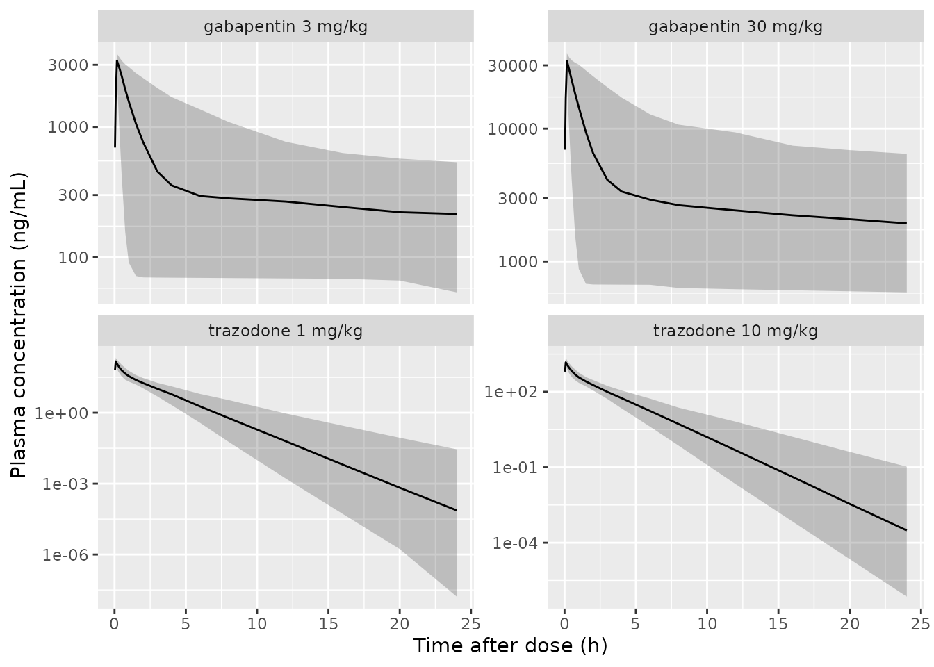
Simulated plasma concentrations in mice (median and 5th-95th percentiles of 200 simulated mice per group).
PKNCA
# Trazodone is ~30 half-lives below its peak by 24 h, where the solver
# can return values of order -1e-7 ng/mL; they are set to zero for the NCA.
conc_pk <- sim_pk |>
  filter(!is.na(conc)) |>
  mutate(conc = pmax(conc, 0)) |>
  select(id, time_h, conc, treatment)
dose_pk <- ev_pk |>
  filter(evid == 1) |>
  transmute(id, time_h = time / 60, amt, treatment)

nca_pk <- PKNCA::pk.nca(PKNCA::PKNCAdata(
  PKNCA::PKNCAconc(conc_pk, conc ~ time_h | treatment + id),
  PKNCA::PKNCAdose(dose_pk, amt ~ time_h | treatment + id),
  intervals = data.frame(start = 0, end = 24, cmax = TRUE, auclast = TRUE)
))
Supplementary Table S6 reports, for the same four dose groups, the NCA of the observed data and the mean of the individual (post-hoc) model predictions. The comparison uses the post-hoc means (Table S6 panels B and D).
published_pk <- tibble::tribble(
  ~treatment,            ~cmax, ~auclast,
  "trazodone 1 mg/kg",     282,     220,
  "trazodone 10 mg/kg",   2156,    1509,
  "gabapentin 3 mg/kg",   3345,    9887,
  "gabapentin 30 mg/kg", 33543,   86130
)
cmp_pk <- nlmixr2lib::ncaComparisonTable(
  simulated = nca_pk,
  reference = published_pk,
  by = "treatment",
  units = c(cmax = "ng/mL", auclast = "ng*h/mL"),
  tolerance_pct = 20
)
knitr::kable(cmp_pk, caption = attr(cmp_pk, "footnote"))| NCA parameter | treatment | Reference | Simulated | % diff |
|---|---|---|---|---|
| Cmax (ng/mL) | trazodone 1 mg/kg | 282 | 149 | -47.0%* |
| Cmax (ng/mL) | trazodone 10 mg/kg | 2160 | 1480 | -31.2%* |
| Cmax (ng/mL) | gabapentin 3 mg/kg | 3340 | 3230 | -3.4% |
| Cmax (ng/mL) | gabapentin 30 mg/kg | 33500 | 32400 | -3.4% |
| AUClast (ng*h/mL) | trazodone 1 mg/kg | 220 | 131 | -40.5%* |
| AUClast (ng*h/mL) | trazodone 10 mg/kg | 1510 | 1350 | -10.8% |
| AUClast (ng*h/mL) | gabapentin 3 mg/kg | 9890 | 9460 | -4.3% |
| AUClast (ng*h/mL) | gabapentin 30 mg/kg | 86100 | 92500 | +7.4% |
Gabapentin agrees with the post-hoc means within about 10%. Trazodone
is lower than the post-hoc means, by about 40-45% at 1 mg/kg and 10-30%
at 10 mg/kg. That gap is in the published estimates rather than in the
simulation: for a linear model the typical AUC is
dose / (k * V1/F), which is 1 / (1.25 x 5.95) = 0.134 mg
h/L = 134 ng h/mL at 1 mg/kg against the reported 220. The observed NCA
(Table S6A: 219 and 1406 ng h/mL) is itself less than dose-proportional,
and the Table 1a values were fitted jointly to 1, 3 and 10 mg/kg, so the
model sits between the low and high doses. The Table 1a values are kept
as published.
Mouse writhing model
Control animals
The acetic acid is given at 60 min, 1 h after the (here absent) drug,
as in the experiments. It is dosed as amt = 1 into
stimulus; the model’s bioavailability
f(stimulus) scales that unit dose to the animal’s stimulus
amplitude S.
n_pd <- 100
pd_times <- seq(60, 120, by = 1)

make_pd_events <- function(groups, n) {
  bind_rows(lapply(seq_len(nrow(groups)), function(i) {
    g <- groups[i, ]
    ids <- (i - 1) * n + seq_len(n)
    bind_rows(
      if (g$trz > 0) data.frame(id = ids, time = 0, amt = g$trz, cmt = "central", evid = 1, rate = -2),
      if (g$gab > 0) data.frame(id = ids, time = 0, amt = g$gab, cmt = "central_gabapentin", evid = 1, rate = -2),
      data.frame(id = ids, time = 60, amt = 1, cmt = "stimulus", evid = 1, rate = 0),
      tidyr::crossing(id = ids, time = pd_times) |>
        mutate(amt = 0, cmt = "writhing", evid = 0, rate = 0)
    ) |>
      mutate(group = g$group)
  })) |>
    arrange(id, time, desc(evid))
}

pd_percentiles <- function(sim) {
  sim |>
    group_by(group, time) |>
    summarise(p05 = quantile(writhing, 0.05), p50 = median(writhing),
              p95 = quantile(writhing, 0.95), .groups = "drop")
}
ctrl <- tibble::tibble(group = "control", trz = 0, gab = 0)
rxode2::rxSetSeed(20230414)
sim_ctrl <- as.data.frame(rxode2::rxSolve(mod_mouse, make_pd_events(ctrl, n_pd),
                                          keep = "group", useLinCmt = FALSE))
pct_ctrl <- pd_percentiles(sim_ctrl)
ggplot(pct_ctrl, aes(time, p50)) +
  geom_ribbon(aes(ymin = p05, ymax = p95), alpha = 0.25) +
  geom_line() +
  labs(x = "Time (min; acetic acid at 60 min)", y = "Number of writhings")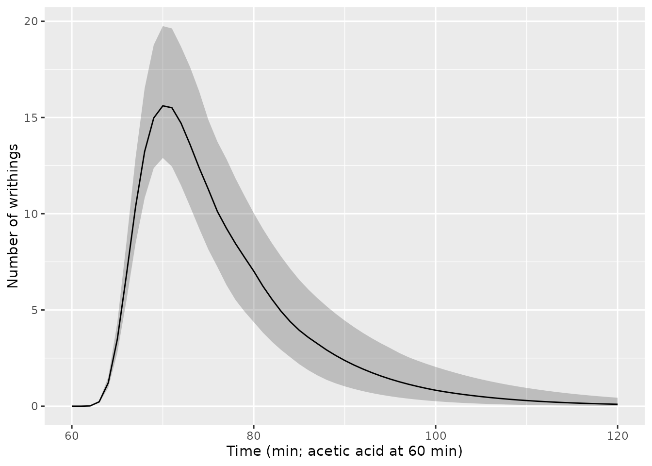
Simulated writhing counts in control mice (median and 5th-95th percentiles of 100 simulated mice; model predictions without residual error).
With the typical values the control curve can be checked against the
structure directly: the stimulus leaves a0 at
ktr, and the writhing count peaks about ten minutes after
the injection.
ev_typ <- make_pd_events(ctrl, 1)
sim_typ <- as.data.frame(rxode2::rxSolve(mod_mouse, ev_typ, omega = NA, sigma = NA,
                                         useLinCmt = FALSE))
t_peak <- sim_typ$time[which.max(sim_typ$writhing)] - 60
w_peak <- max(sim_typ$writhing)
c(t_peak_min = t_peak, peak_writhings = round(w_peak, 2))
#>     t_peak_min peak_writhings
#>          10.00          16.42
# A total stimulus S passes through the chain, so the area under W over all
# time is S / k. The 60-minute grid captures nearly all of it.
auc_w <- sum(diff(sim_typ$time) * (head(sim_typ$writhing, -1) + tail(sim_typ$writhing, -1)) / 2)
stopifnot(t_peak >= 9, t_peak <= 12, abs(auc_w / (26.10 / 0.104) - 1) < 0.05)
Replication of Figure 1: combinations under additivity
Figure 1 simulates 100 mice for each combination group assuming
additivity. The single-agent potencies of Table 3 are used here with
gamma = 0.
mod_additive_t3 <- mod_mouse |>
  rxode2::ini(
    lslope = log(10.9), lslope_gabapentin = log(0.0459), synergy = 0,
    etalslope ~ 1.42, etalslope_gabapentin ~ 1.97
  )
combos <- tibble::tribble(
  ~group,                                  ~trz,  ~gab,
  "(a) 0.075 mg/kg TRZ + 1.5 mg/kg GBP",  0.075,  1.5,
  "(b) 0.15 mg/kg TRZ + 1.5 mg/kg GBP",   0.15,   1.5,
  "(c) 0.5 mg/kg TRZ + 5 mg/kg GBP",      0.5,    5,
  "(d) 1.5 mg/kg TRZ + 15 mg/kg GBP",     1.5,    15
)
rxode2::rxSetSeed(20230415)
sim_fig1 <- as.data.frame(rxode2::rxSolve(mod_additive_t3, make_pd_events(combos, n_pd),
                                          keep = "group", useLinCmt = FALSE))
pct_fig1 <- pd_percentiles(sim_fig1)
ggplot(pct_fig1, aes(time)) +
  geom_line(aes(y = p50), colour = "red", linewidth = 1) +
  geom_line(aes(y = p05), colour = "red") +
  geom_line(aes(y = p95), colour = "red") +
  facet_wrap(~group, scales = "free_y") +
  labs(x = "Time (min)", y = "Number of writhings")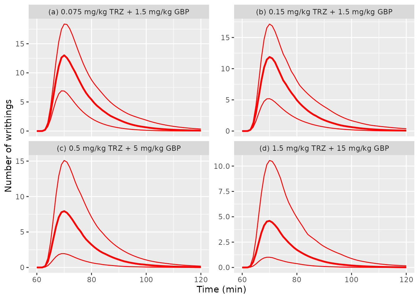
Replicates Figure 1 of Oggianu 2023: simulated writhings (5th, 50th and 95th percentiles of 100 mice) for the four combinations under additivity, using the Table 3 single-agent potencies.
The published panels peak near 70 min with a median of roughly 12, 11, 6.5 and 3 writhings for panels (a)-(d) and a 95th percentile of roughly 17, 18, 14 and 10 (read from the figure by the maintainers). The simulated peak percentiles are:
fig1_peak <- pct_fig1 |>
  group_by(group) |>
  slice_max(p50, n = 1, with_ties = FALSE) |>
  ungroup() |>
  mutate(figure_p50 = c(12, 11, 6.5, 3), figure_p95 = c(17, 18, 14, 10))
fig1_peak |>
  transmute(
    "Group" = group,
    "Peak time (min)" = time,
    "Simulated 5th" = round(p05, 1),
    "Simulated median" = round(p50, 1),
    "Figure 1 median (approx.)" = figure_p50,
    "Simulated 95th" = round(p95, 1),
    "Figure 1 95th (approx.)" = figure_p95
  ) |>
knitr::kable()| Group | Peak time (min) | Simulated 5th | Simulated median | Figure 1 median (approx.) | Simulated 95th | Figure 1 95th (approx.) |
|---|---|---|---|---|---|---|
| (a) 0.075 mg/kg TRZ + 1.5 mg/kg GBP | 70 | 6.9 | 13.0 | 12.0 | 18.4 | 17 |
| (b) 0.15 mg/kg TRZ + 1.5 mg/kg GBP | 70 | 5.2 | 11.9 | 11.0 | 17.2 | 18 |
| (c) 0.5 mg/kg TRZ + 5 mg/kg GBP | 70 | 2.0 | 7.9 | 6.5 | 15.1 | 14 |
| (d) 1.5 mg/kg TRZ + 15 mg/kg GBP | 70 | 1.0 | 4.6 | 3.0 | 10.6 | 10 |
# Structural check: the higher-dose combinations suppress writhing more.
stopifnot(
  fig1_peak$p50[3] < fig1_peak$p50[1],
  fig1_peak$p50[4] < fig1_peak$p50[3]
)
The simulated peak medians and 95th percentiles fall within about 1.5 writhings of the published panels.
Additive versus synergic fits (Tables 4 and 5)
For the two low-dose combinations the synergic model (Table 4B, the
packaged parameters) lowered the objective function by 17 points
relative to the additive model (Table 4A). The typical-value writhing
areas over the 30-min counting window show what gamma
adds:
mod_additive_t4a <- mod_mouse |>
  rxode2::ini(lslope = log(12.7), lslope_gabapentin = log(0.0808), synergy = 0)
mod_additive_t5a <- mod_mouse |>
  rxode2::ini(lslope = log(10.2), lslope_gabapentin = log(0.040), synergy = 0)
low_high <- tibble::tribble(
  ~group,                                ~trz,   ~gab,
  "control",                             0,      0,
  "0.075 mg/kg TRZ + 1.5 mg/kg GBP",    0.075,  1.5,
  "0.15 mg/kg TRZ + 1.5 mg/kg GBP",     0.15,   1.5,
  "0.5 mg/kg TRZ + 5 mg/kg GBP",        0.5,    5,
  "1.5 mg/kg TRZ + 15 mg/kg GBP",       1.5,    15
)
ev_lh <- make_pd_events(low_high, 1) |> filter(time <= 90)
w_area <- function(m) {
  as.data.frame(rxode2::rxSolve(m, ev_lh, omega = NA, sigma = NA, keep = "group",
                                useLinCmt = FALSE)) |>
    group_by(group) |>
    summarise(area = sum(diff(time) * (head(writhing, -1) + tail(writhing, -1)) / 2),
              .groups = "drop")
}
syn_tab <- w_area(mod_mouse) |>
  rename(synergic_4B = area) |>
  left_join(rename(w_area(mod_additive_t4a), additive_4A = area), by = "group") |>
  left_join(rename(w_area(mod_additive_t5a), additive_5A = area), by = "group")
ctrl_area <- syn_tab$synergic_4B[syn_tab$group == "control"]
syn_tab |>
  mutate(across(-group, ~ round(100 * (1 - .x / ctrl_area), 1))) |>
  filter(group != "control") |>
  rename(
    "Group" = group,
    "% inhibition, synergic (Table 4B)" = synergic_4B,
    "% inhibition, additive (Table 4A)" = additive_4A,
    "% inhibition, additive (Table 5A)" = additive_5A
  ) |>
knitr::kable()| Group | % inhibition, synergic (Table 4B) | % inhibition, additive (Table 4A) | % inhibition, additive (Table 5A) |
|---|---|---|---|
| 0.075 mg/kg TRZ + 1.5 mg/kg GBP | 37.2 | 24.1 | 15.2 |
| 0.15 mg/kg TRZ + 1.5 mg/kg GBP | 51.0 | 28.1 | 19.2 |
| 0.5 mg/kg TRZ + 5 mg/kg GBP | 90.5 | 56.7 | 44.3 |
| 1.5 mg/kg TRZ + 15 mg/kg GBP | 98.8 | 79.7 | 70.5 |
The synergy estimate comes from the two low-dose combinations only.
At the high-dose combinations the authors found gamma
indistinguishable from zero (Table 5B, gamma = 0.0001), so
the packaged gamma = 16 overstates the interaction there;
use rxode2::ini(mod, synergy = 0) with the Table 5
potencies for doses at or above 0.5 + 5 mg/kg.
Human trazodone
Pharmacokinetics (Supplementary Table S3)
Table S3 reports the simulated AUC from time zero to infinity after
single oral trazodone doses of 0.5-50 mg, and the same AUC rescaled for
protein binding (AUCeq).
mod_human <- readModelDb("Oggianu_2023_trazodone_human")
hum_doses <- c(0.5, 1, 5, 10, 25, 50)
n_hum <- 200
hum_times <- c(0, 0.083, 0.167, 0.25, 0.5, 0.75, 1, 1.5, 2, 3, 4, 6, 8, 12, 16, 24, 36, 48, 72)
ev_hum <- bind_rows(lapply(seq_along(hum_doses), function(i) {
  ids <- (i - 1) * n_hum + seq_len(n_hum)
  bind_rows(
    data.frame(id = ids, time = 0, amt = hum_doses[i], cmt = "depot", evid = 1),
    tidyr::crossing(id = ids, time = hum_times) |>
      mutate(amt = 0, cmt = "central", evid = 0)
  ) |>
    mutate(treatment = paste(hum_doses[i], "mg"))
})) |>
  arrange(id, time, desc(evid))

rxode2::rxSetSeed(20230416)
sim_hum <- as.data.frame(rxode2::rxSolve(mod_human, ev_hum, keep = "treatment"))
#> ℹ parameter labels from comments will be replaced by 'label()'

nca_hum <- PKNCA::pk.nca(PKNCA::PKNCAdata(
  PKNCA::PKNCAconc(filter(sim_hum, !is.na(Cc)), Cc ~ time | treatment + id),
  PKNCA::PKNCAdose(filter(ev_hum, evid == 1), amt ~ time | treatment + id),
  intervals = data.frame(start = 0, end = Inf, aucinf.obs = TRUE)
))
published_hum <- tibble::tibble(
  treatment = paste(hum_doses, "mg"),
  aucinf.obs = c(46.1, 92.7, 458, 931, 2323, 4643)
)
cmp_hum <- nlmixr2lib::ncaComparisonTable(
  simulated = nca_hum,
  reference = published_hum,
  by = "treatment",
  units = c(aucinf.obs = "ng*h/mL"),
  tolerance_pct = 20
)
knitr::kable(cmp_hum, caption = attr(cmp_hum, "footnote"))| NCA parameter | treatment | Reference | Simulated | % diff |
|---|---|---|---|---|
| AUC0-∞ (obs) (ng*h/mL) | 0.5 mg | 46.1 | 50.5 | +9.6% |
| AUC0-∞ (obs) (ng*h/mL) | 1 mg | 92.7 | 96.1 | +3.6% |
| AUC0-∞ (obs) (ng*h/mL) | 5 mg | 458 | 518 | +13.1% |
| AUC0-∞ (obs) (ng*h/mL) | 10 mg | 931 | 1030 | +10.9% |
| AUC0-∞ (obs) (ng*h/mL) | 25 mg | 2320 | 2550 | +9.9% |
| AUC0-∞ (obs) (ng*h/mL) | 50 mg | 4640 | 4960 | +6.7% |
The reference values are the Table S3 medians. The typical-value AUC
is dose / (CL/F) = 50.7 ng h/mL at 0.5 mg, about 10% above
the published median of 46.1; the published simulation’s median-to-dose
ratio is constant across doses (92.2-92.9 ng h/mL per mg), so the gap is
a fixed scale offset rather than nonlinearity. The AUCeq
column of Table S3 is AUC x (1 - 0.97) / (1 - 0.89), the
same factor the model applies before the concentration drives the
writhing layer:
fu_ratio <- (1 - 0.97) / (1 - 0.89)
table_s3 <- tibble::tibble(
  dose = hum_doses,
  auc_tot_mean = c(48.1, 96.3, 481, 967, 2438, 4784),
  auc_eq_mean = c(13.1, 26.3, 131, 264, 665, 1305)
)
table_s3 |>
  mutate(ratio = round(auc_eq_mean / auc_tot_mean, 4)) |>
knitr::kable()| dose | auc_tot_mean | auc_eq_mean | ratio |
|---|---|---|---|
| 0.5 | 48.1 | 13.1 | 0.2723 |
| 1.0 | 96.3 | 26.3 | 0.2731 |
| 5.0 | 481.0 | 131.0 | 0.2723 |
| 10.0 | 967.0 | 264.0 | 0.2730 |
| 25.0 | 2438.0 | 665.0 | 0.2728 |
| 50.0 | 4784.0 | 1305.0 | 0.2728 |
Translation of the writhing effect (Table 6, trazodone alone)
The paper’s design is replicated for each virtual subject: the
stimulus is first applied without drug, the compartments are reset
(evid = 3), and the stimulus is applied again 1 h after a
trazodone dose. Percent inhibition is one minus the ratio of the two
writhing areas over the 30-min counting window. Both phases share the
subject’s parameters, so the comparison is within subject, as in the
paper.
grid_30 <- seq(0, 0.5, by = 1 / 120)
ev_tr <- bind_rows(lapply(seq_along(hum_doses), function(i) {
  ids <- (i - 1) * n_hum + seq_len(n_hum)
  bind_rows(
    data.frame(id = ids, time = 0, amt = 1, cmt = "stimulus", evid = 1),
    tidyr::crossing(id = ids, time = grid_30) |> mutate(amt = 0, cmt = "writhing", evid = 0),
    data.frame(id = ids, time = 24, amt = 0, cmt = "writhing", evid = 3),
    data.frame(id = ids, time = 24, amt = hum_doses[i], cmt = "depot", evid = 1),
    data.frame(id = ids, time = 25, amt = 1, cmt = "stimulus", evid = 1),
    tidyr::crossing(id = ids, time = 25 + grid_30) |> mutate(amt = 0, cmt = "writhing", evid = 0)
  ) |>
    mutate(dose = hum_doses[i])
})) |>
  arrange(id, time, desc(evid))

rxode2::rxSetSeed(20230417)
sim_tr <- as.data.frame(rxode2::rxSolve(mod_human, ev_tr, keep = "dose"))
inh <- sim_tr |>
  mutate(phase = ifelse(time < 24, "no_drug", "drug")) |>
  group_by(id, dose, phase) |>
  summarise(area = sum(diff(time) * (head(writhing, -1) + tail(writhing, -1)) / 2),
            .groups = "drop") |>
  tidyr::pivot_wider(names_from = phase, values_from = area) |>
  mutate(pct_inh = 100 * (1 - drug / no_drug))

table6 <- tibble::tibble(
  dose = hum_doses,
  paper_mean = c(4.93, 9.20, 27.6, 37.5, 56.2, 69.41),
  paper_median = c(2.76, 5.67, 21.7, 34.1, 58.7, 73.96),
  paper_q1 = c(1.18, 2.50, 10.5, 18.6, 38.4, 55.09),
  paper_q3 = c(6.03, 11.75, 39.6, 53.3, 75.0, 85.97)
)
inh_sum <- inh |>
  group_by(dose) |>
  summarise(sim_mean = mean(pct_inh), sim_median = median(pct_inh),
            sim_q1 = quantile(pct_inh, 0.25), sim_q3 = quantile(pct_inh, 0.75)) |>
  left_join(table6, by = "dose")
inh_sum |>
  transmute(
    "Trazodone dose (mg)" = dose,
    "Mean, paper" = paper_mean, "Mean, simulated" = round(sim_mean, 1),
    "Median, paper" = paper_median, "Median, simulated" = round(sim_median, 1),
    "Q1, paper" = paper_q1, "Q1, simulated" = round(sim_q1, 1),
    "Q3, paper" = paper_q3, "Q3, simulated" = round(sim_q3, 1)
  ) |>
knitr::kable(caption = "Percent inhibition of the pain stimulus after single oral trazodone doses (Table 6, gabapentin 0 mg column).")| Trazodone dose (mg) | Mean, paper | Mean, simulated | Median, paper | Median, simulated | Q1, paper | Q1, simulated | Q3, paper | Q3, simulated |
|---|---|---|---|---|---|---|---|---|
| 0.5 | 4.93 | 5.0 | 2.76 | 3.2 | 1.18 | 1.5 | 6.03 | 6.6 |
| 1.0 | 9.20 | 10.5 | 5.67 | 6.5 | 2.50 | 2.8 | 11.75 | 14.5 |
| 5.0 | 27.60 | 27.4 | 21.70 | 22.3 | 10.50 | 11.6 | 39.60 | 38.4 |
| 10.0 | 37.50 | 43.9 | 34.10 | 41.0 | 18.60 | 25.2 | 53.30 | 61.4 |
| 25.0 | 56.20 | 59.4 | 58.70 | 59.6 | 38.40 | 42.2 | 75.00 | 78.3 |
| 50.0 | 69.41 | 72.4 | 73.96 | 76.1 | 55.09 | 62.2 | 85.97 | 88.3 |
# Centre-of-distribution checks across the six doses. With a 119% CV on the
# potency, a 200-subject mean moves by several points between cohorts, so
# the check is on the median difference across doses, not on any one dose.
stopifnot(
  abs(median(inh_sum$sim_median - inh_sum$paper_median)) < 4,
  abs(median(inh_sum$sim_mean - inh_sum$paper_mean)) < 4
)
ggplot(inh_sum, aes(dose)) +
  geom_ribbon(aes(ymin = sim_q1, ymax = sim_q3), alpha = 0.25) +
  geom_line(aes(y = sim_median)) +
  geom_pointrange(aes(y = paper_median, ymin = paper_q1, ymax = paper_q3), colour = "red") +
  scale_x_log10() +
  labs(x = "Trazodone dose (mg)", y = "Inhibition of writhing stimulus (%)")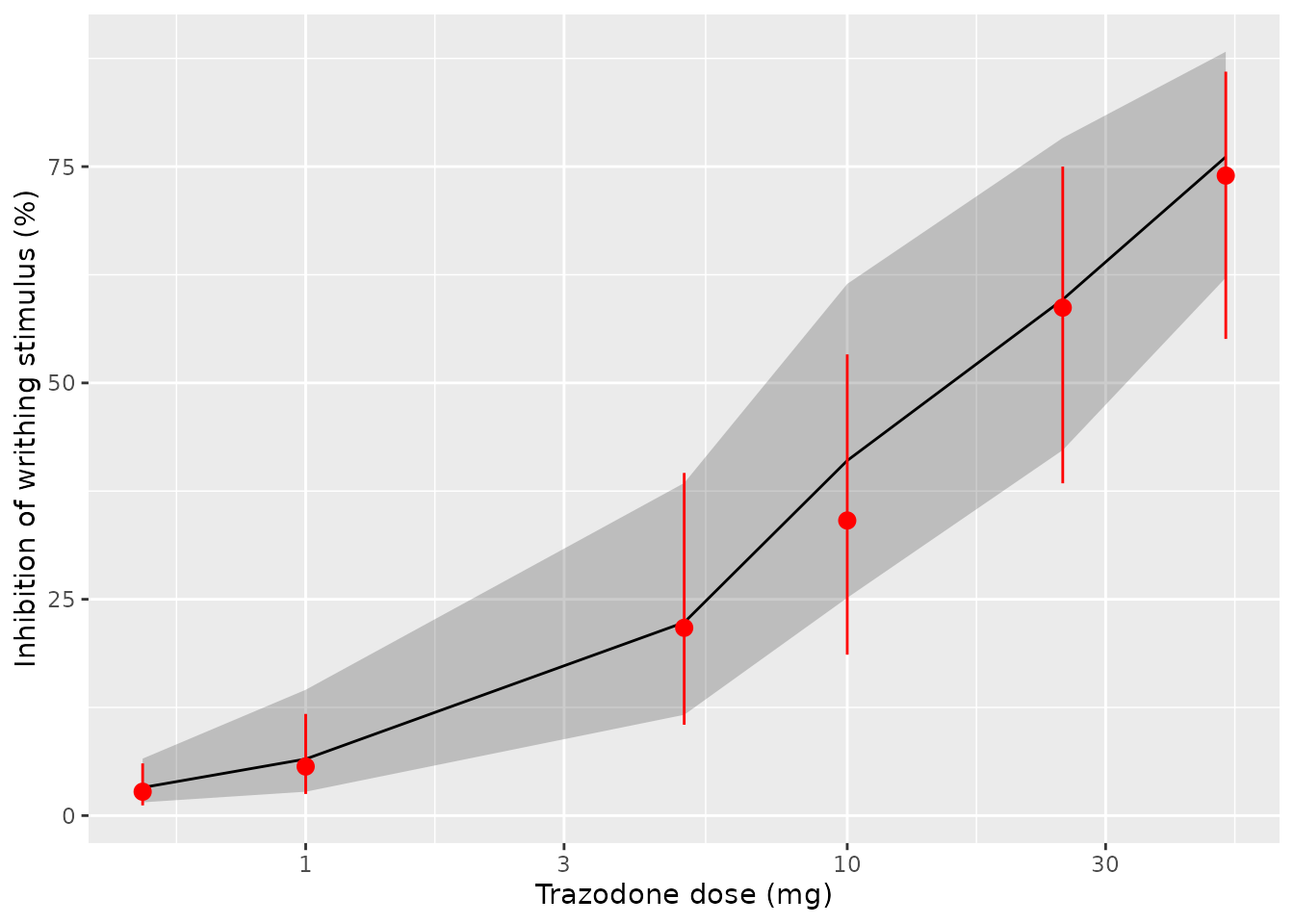
Percent inhibition of the writhing stimulus versus human trazodone dose: simulated median and interquartile range (line and band) against the Table 6 values (points and error bars).
The gabapentin columns of Table 6 (gabapentin alone and with trazodone) need the human gabapentin model of Carlsson et al. (2009), which this paper uses but does not reprint, so they are not reproduced here.
Assumptions and deviations
-
Time units. The mouse model runs in minutes because
the writhing parameters are per minute; the mouse PK parameters keep
their published hour units in
ini()and are divided by 60 inmodel(). The human model runs in hours and multiplies the per-minute writhing parameters by 60. -
Molar conversion. The potencies
k2are per umol/L, so the plasma concentration is divided by the free-base molecular weight (trazodone 371.86, gabapentin 171.24 g/mol). The molecular weights are not printed in the paper. The Table 6 reproduction above depends on this conversion and agrees with the published values. -
Stimulus as a dose. The paper gives the stimulus as
the initial condition
a0(0) = S. Because the drugs are given 1 h earlier, the model doses the stimulus asamt = 1intostimulusat the time of the acetic acid, withf(stimulus) = S. -
Number of transit compartments. Table 2 reports
n = 9with an interindividual variance (omega2 n = 0.00848). The PK/PD equations of Supplementary Table S1B write the chain as nine explicit compartments, and an explicit chain cannot carry a random number of compartments, so the model follows the printed equations withn = 9for every animal and omitsomega2 n. - Packaged drug-effect parameters. The mouse model carries the Table 4B synergic fit. It was estimated on the two low-dose combinations; at the high-dose combinations the authors found additivity (Table 5). The Table 3 single-agent fits had separate additive residual variances (3.20 and 2.17); the model carries the single Table 4B value (2.64).
-
Sequential estimation. The PK parameters and the
control-group PD parameters were estimated first and held fixed while
the potencies and
gammawere estimated. They are not wrapped infixed(), because they are estimates from this paper. The zero-order input durationsD1(5 and 10 min) have no reported standard error and are encoded as fixed. -
Human translation. The writhing parameters in the
human model are the mouse estimates and are wrapped in
fixed(); the trazodone potency is assumed equal across species, as the paper states. Human concentrations are scaled by the unbound-fraction ratio (1 - 0.97) / (1 - 0.89) before they act. The per-subject percent inhibition uses the 30-min counting window of the mouse experiment; the paper does not state the window used for the human areas, and integrating the full writhing curve instead changes the percentages by a fraction of a percentage point. - Trazodone mouse exposure. The typical-value trazodone AUC and Cmax are below the post-hoc means of Table S6 (see the PKNCA section); the Table 1a values are used as published.
- Human gabapentin. The human gabapentin PK model (Carlsson et al., Ther Drug Monit 2009;31:86-94) is cited but not reprinted, so the human model covers trazodone only.
-
Animal numbers. The total number of mice in the
writhing experiments is not reported (6-9 per group), so
n_subjectsisNAin the mouse model.