Vancomycin (Garreau 2021)
Source:vignettes/articles/Garreau_2021_vancomycin.Rmd
Garreau_2021_vancomycin.RmdModel and source
- Citation: Garreau R, Falquet B, Mioux L, Bourguignon L, Ferry T, Tod M, Wallet F, Friggeri A, Richard JC, Goutelle S. Population Pharmacokinetics and Dosing Simulation of Vancomycin Administered by Continuous Injection in Critically Ill Patient. Antibiotics (Basel). 2021;10(10):1228. doi:10.3390/antibiotics10101228
- Description: Two-compartment IV population PK model for vancomycin given by continuous infusion to 78 critically ill adults in intensive care, 22 of them on continuous renal replacement therapy (Garreau 2021). Clearance depends on Cockcroft-Gault creatinine clearance (ideal-body-weight based) in patients off CRRT and on the CRRT effluent flow rate in patients on CRRT; the central volume depends on ideal body weight. As printed in the paper’s final-model equations, each covariate enters as the exponential of a centred power term, CL = CLpop * exp((CRCL/41.4)^0.5), rather than as the plain power form of the Methods. Proportional residual error.
- Article: https://doi.org/10.3390/antibiotics10101228 (open access, CC BY 4.0)
Population
Garreau 2021 built the model from a learning dataset collected at the Croix-Rousse Hospital (University Hospitals of Lyon, France) between December 2013 and April 2015: 78 critically ill adults in intensive care who received vancomycin by continuous infusion and had invasive PiCCO haemodynamic monitoring, contributing 335 concentrations from routine morning therapeutic drug monitoring over 4.1 +/- 2 days. Baseline characteristics (Table 1): 57 men and 21 women, age 68.9 +/- 12.3 years, total body weight 77.9 +/- 20.4 kg, ideal body weight (Devine) 63.5 +/- 9 kg, height 168.7 +/- 8.5 cm, SOFA 11 +/- 4, IGS-II 55.9 +/- 17.3, septic shock in 83.3%, serum creatinine 139.3 +/- 75.7 umol/L and Cockcroft-Gault creatinine clearance 50.4 +/- 29 mL/min. Twenty-two patients (28.2%) were on continuous renal replacement therapy (CRRT) with an effluent flow of 35.6 +/- 18.7 mL/min. The mean loading dose was 22.7 +/- 7.5 mg/kg and the mean maintenance dose 28.6 +/- 9.4 mg/kg/day.
An external validation set from a second Lyon centre (84 patients, 417 concentrations, 4 on CRRT) was used only to evaluate predictive performance (Figure 3) and did not inform the estimates.
The same information is available programmatically via
readModelDb("Garreau_2021_vancomycin")()$population.
Source trace
The per-parameter origin is recorded as an in-file comment next to
each ini() entry in
inst/modeldb/specificDrugs/Garreau_2021_vancomycin.R. The
table below collects them in one place.
| Equation / parameter | Value | Source location |
|---|---|---|
lcl (CLpop) |
log(0.79) L/h |
Table 2, CLpop (RSE 12.7%) |
lvc (V1pop) |
log(27.3) L |
Table 2, V1pop (RSE 45.1%) |
lq (Qpop) |
log(6.08) L/h |
Table 2, Qpop (RSE 41.8%); Sect. 2.2 rounds to 6.1 |
lvp (V2pop) |
log(61.3) L |
Table 2, V2pop (RSE 9.7%); Sect. 2.2 prose prints 63.1
(digit transposition; table used) |
e_ibw_vc (alpha) |
1.88 |
Table 2, alpha (RSE 67.1%) |
e_crcl_cl |
fixed(0.5) |
Table 2 final-model equation,
CL0 = CLpop e^((CRCL/41.4)^0.5) if CRRT = 0 |
e_rrt_crrt_effluent_flow_cl |
fixed(0.69) |
Table 2 final-model equation,
CL0 = CLpop e^((CRRTEFR/20)^0.69) if CRRT = 1 |
etalcl |
0.76^2 = 0.5776 |
Table 2, omega_CL = 0.76 (SD; RSE 11.1%) |
etalvc |
0.61^2 = 0.3721 |
Table 2, omega_V = 0.61 (SD; RSE 51.1%) |
etalq |
0.49^2 = 0.2401 |
Table 2, omega_Q = 0.49 (SD; RSE 33.8%) |
etalvp |
0.48^2 = 0.2304 |
Table 2, omega_V2 = 0.48 (SD; RSE 16.5%) |
propSd |
0.13 |
Table 2, residual b = 0.13 (RSE 6.3%); proportional
error per Sect. 2.2 |
| CL covariate model | cl <- exp(lcl + etalcl) * [(1 - CRRT) exp((CRCL/41.4)^0.5) + CRRT exp((EFR/1200)^0.69)] |
Table 2 final-model equations (effluent flow in mL/h; 20 mL/min = 1200 mL/h) |
| V1 covariate model | vc <- exp(lvc + etalvc) * exp((IBW/64.1)^e_ibw_vc) |
Table 2 final-model equation |
| Q, V2 |
exp(lq + etalq), exp(lvp + etalvp)
|
Table 2 final-model equations (no covariates) |
| Structure | two compartments, IV input into central | Sect. 2.2, “a two-compartment model with a proportional residual error” |
| CRCL definition | Cockcroft-Gault on IBW, mL/min; 0 when on CRRT or anuric | Sect. 4.1; Discussion (“CRCL based on IBW”, “CG_IBW”) |
The covariate equations: exponential of a centred power term
The paper prints the covariate model in two places, and the two do not agree.
-
Methods Eq. (1) gives the generic
continuous-covariate form
X = Xpop * (COV / COVmedian)^alpha, the plain power model. -
The Table 2 final-model equations place the centred
power term inside an exponential:
CL0 = CLpop * e^((CRCL/41.4)^0.5),CL0 = CLpop * e^((CRRTEFR/20)^0.69)andV1 = V1pop * e^((IBW/64.1)^alpha) * e^eta. The exponential is not a PDF rendering artefact: the article’s JATS MathML nests the power term inside an<msup>whose base ise, for all three equations.
The model file follows the Table 2 equations. They are the specific
statement of the final model, and Eq. (1) describes the general form
tried during covariate building. The data also rule out the plain power
form for clearance. It would give a typical clearance of
0.79 * sqrt(50.4 / 41.4) = 0.87 L/h at the cohort’s mean
CRCL. At the cohort’s mean maintenance dose of 28.6 mg/kg/day, that
clearance gives a steady-state concentration of about 100 mg/L. Every
population prediction in Figure 1 lies between about 5 and 55 mg/L. The
exponential form gives 2.4 L/h and about 40 mg/L. The chunk below
reproduces this arithmetic.
mean_crcl <- 50.4 # Table 1, mL/min
mean_tbw <- 77.9 # Table 1, kg
mean_md <- 28.6 # Table 1, mg/kg/day (maintenance)
rate_mgh <- mean_md * mean_tbw / 24

cl_printed <- 0.79 * exp((mean_crcl / 41.4)^0.5)
cl_eq1 <- 0.79 * (mean_crcl / 41.4)^0.5
form_tab <- tibble::tibble(
  Form = c("Table 2 printed: exp of power", "Methods Eq. (1): plain power"),
  `CL (L/h)` = signif(c(cl_printed, cl_eq1), 3),
  `Css (mg/L)` = signif(rate_mgh / c(cl_printed, cl_eq1), 3)
)
knitr::kable(form_tab)| Form | CL (L/h) | Css (mg/L) |
|---|---|---|
| Table 2 printed: exp of power | 2.380 | 39 |
| Methods Eq. (1): plain power | 0.872 | 107 |
# Figure 1 (population predictions, learning set) spans about 5-55 mg/L. The
# printed form lands inside it; the power form lands far outside it.
stopifnot(
  rate_mgh / cl_printed > 5, rate_mgh / cl_printed < 55,
  rate_mgh / cl_eq1 > 90
)
As a consequence, CLpop and V1pop are
not the clearance and central volume of a reference
patient. A patient off CRRT with CRCL = 41.4 mL/min has
CL = 0.79 * e = 2.15 L/h; a patient on CRRT at 20 mL/min
effluent has the same 2.15 L/h; an anuric patient off CRRT (CRCL = 0)
keeps CL = 0.79 L/h. A patient with IBW = 64.1 kg has
V1 = 27.3 * e = 74.2 L.
mod <- readModelDb("Garreau_2021_vancomycin")
mod_typ <- rxode2::zeroRe(mod)
#> ℹ parameter labels from comments will be replaced by 'label()'

id_cov <- tibble::tribble(
  ~case,                         ~CRCL, ~IBW, ~RRT_CRRT_STATUS, ~RRT_CRRT_EFFLUENT_FLOW, ~cl_expected,        ~vc_expected,
  "Off CRRT, CRCL 41.4",          41.4,  64.1, 0,                0,                       0.79 * exp(1),       27.3 * exp(1),
  "Off CRRT, CRCL 0 (anuric)",     0,    64.1, 0,                0,                       0.79,                27.3 * exp(1),
  "Off CRRT, CRCL 120",           120,   50,   0,                0,                       0.79 * exp(sqrt(120 / 41.4)), 27.3 * exp((50 / 64.1)^1.88),
  "On CRRT, effluent 20 mL/min",   0,    64.1, 1,                1200,                    0.79 * exp(1),       27.3 * exp(1),
  "On CRRT, effluent 35.6 mL/min", 0,    80,   1,                35.6 * 60,               0.79 * exp((35.6 / 20)^0.69), 27.3 * exp((80 / 64.1)^1.88)
)

id_ev <- id_cov |>
  dplyr::mutate(id = dplyr::row_number(), time = 0, amt = 0, evid = 2, cmt = "central") |>
  dplyr::select(id, time, amt, evid, cmt, CRCL, IBW, RRT_CRRT_STATUS, RRT_CRRT_EFFLUENT_FLOW)
id_sim <- rxode2::rxSolve(mod_typ, events = id_ev, returnType = "data.frame") |>
  dplyr::distinct(id, .keep_all = TRUE)
#> ℹ omega/sigma items treated as zero: 'etalcl', 'etalvc', 'etalq', 'etalvp'
#> Warning: multi-subject simulation without without 'omega'

id_tab <- id_cov |>
  dplyr::mutate(cl_model = id_sim$cl, vc_model = id_sim$vc)
knitr::kable(
  id_tab |>
    dplyr::select(case, cl_expected, cl_model, vc_expected, vc_model) |>
    dplyr::mutate(dplyr::across(where(is.numeric), \(x) signif(x, 5))) |>
    dplyr::rename(
      Case = case, `CL expected (L/h)` = cl_expected, `CL model (L/h)` = cl_model,
      `V1 expected (L)` = vc_expected, `V1 model (L)` = vc_model
    )
)| Case | CL expected (L/h) | CL model (L/h) | V1 expected (L) | V1 model (L) |
|---|---|---|---|---|
| Off CRRT, CRCL 41.4 | 2.1474 | 2.1474 | 74.209 | 74.209 |
| Off CRRT, CRCL 0 (anuric) | 0.7900 | 0.7900 | 74.209 | 74.209 |
| Off CRRT, CRCL 120 | 4.3353 | 4.3353 | 51.098 | 51.098 |
| On CRRT, effluent 20 mL/min | 2.1474 | 2.1474 | 74.209 | 74.209 |
| On CRRT, effluent 35.6 mL/min | 3.5005 | 3.5005 | 124.420 | 124.420 |
Steady state under continuous infusion
Under a continuous infusion at rate R, the steady-state
concentration of a linear two-compartment model is R / CL,
independent of the volumes. This checks the ODE system against its
closed form for a range of covariate profiles.
ss_cov <- tibble::tibble(
  CRCL = c(10, 41.4, 90, 150, 0, 0),
  IBW = c(55, 64.1, 70, 60, 64.1, 75),
  RRT_CRRT_STATUS = c(0, 0, 0, 0, 1, 1),
  RRT_CRRT_EFFLUENT_FLOW = c(0, 0, 0, 0, 20 * 60, 30 * 60)
) |>
  dplyr::mutate(id = dplyr::row_number(), rate = 25 * IBW / 24)

ss_ev <- dplyr::bind_rows(
  ss_cov |> dplyr::mutate(time = 0, amt = rate * 2000, evid = 1, cmt = "central"),
  ss_cov |> dplyr::mutate(time = 1500, amt = 0, evid = 0, rate = 0, cmt = "central")
) |>
  dplyr::arrange(id, time)

ss_sim <- rxode2::rxSolve(
  mod_typ,
  events = ss_ev, rtol = 1e-10, atol = 1e-12, maxsteps = 1e6,
  returnType = "data.frame"
)
#> ℹ omega/sigma items treated as zero: 'etalcl', 'etalvc', 'etalq', 'etalvp'
#> Warning: multi-subject simulation without without 'omega'
ss_chk <- ss_sim |>
  dplyr::filter(time == 1500) |>
  dplyr::left_join(ss_cov |> dplyr::select(id, rate), by = "id") |>
  dplyr::mutate(css_closed = rate / cl, rel_err = Cc / css_closed - 1)
knitr::kable(
  ss_chk |>
    dplyr::select(id, cl, Cc, css_closed, rel_err) |>
    dplyr::mutate(dplyr::across(c(cl, Cc, css_closed), \(x) signif(x, 5))) |>
    dplyr::rename(
      Subject = id, `CL (L/h)` = cl, `Simulated Css (mg/L)` = Cc,
      `R/CL (mg/L)` = css_closed, `Relative error` = rel_err
    )
)| Subject | CL (L/h) | Simulated Css (mg/L) | R/CL (mg/L) | Relative error |
|---|---|---|---|---|
| 1 | 1.2914 | 44.363 | 44.363 | -2e-07 |
| 2 | 2.1474 | 31.093 | 31.093 | 0e+00 |
| 3 | 3.4511 | 21.128 | 21.128 | 0e+00 |
| 4 | 5.3002 | 11.792 | 11.792 | 0e+00 |
| 5 | 2.1474 | 31.093 | 31.093 | 0e+00 |
| 6 | 2.9657 | 26.343 | 26.343 | 0e+00 |
Virtual cohort for the dosing simulations (Table 3)
Section 4.3 and the Table 3 footnote describe the simulated regimens:
a loading dose of 27.5 mg/kg of IBW over 2 h, then a maintenance
continuous infusion in mg/kg of IBW per 24 h, with the endpoint
AUC24-48. Each of the 15 CRCL strata (10 to 150 mL/min) and
the two CRRT effluent strata (20 and 30 mL/min) receives its Table 3
“optimal” maintenance dose. The paper does not describe the IBW
distribution of its virtual patients. IBW is drawn from the learning-set
summary (mean 63.5 kg, SD 9 kg), redrawing any value outside 45-85
kg.
rxode2::rxSetSeed(20211009)
n_per_arm <- 200L # cap is 200 per arm

tab3 <- tibble::tribble(
  ~stratum,       ~CRCL, ~RRT_CRRT_STATUS, ~efr_mlmin, ~md,  ~auc_pub, ~auc_lo, ~auc_hi, ~pta400, ~pta_band, ~pta600,
  "CRCL 150",       150, 0,  0, 30,   493, 330, 644, 0.80, 0.64, 0.16,
  "CRCL 140",       140, 0,  0, 30,   506, 335, 666, 0.83, 0.62, 0.21,
  "CRCL 130",       130, 0,  0, 27.5, 483, 316, 643, 0.77, 0.63, 0.14,
  "CRCL 120",       120, 0,  0, 27.5, 499, 324, 668, 0.80, 0.61, 0.19,
  "CRCL 110",       110, 0,  0, 25,   475, 303, 646, 0.74, 0.60, 0.14,
  "CRCL 100",       100, 0,  0, 25,   492, 313, 674, 0.77, 0.58, 0.19,
  "CRCL 90",         90, 0,  0, 25,   508, 320, 704, 0.80, 0.55, 0.25,
  "CRCL 80",         80, 0,  0, 22.5, 484, 298, 684, 0.75, 0.56, 0.19,
  "CRCL 70",         70, 0,  0, 22.5, 503, 307, 720, 0.78, 0.55, 0.23,
  "CRCL 60",         60, 0,  0, 20,   486, 287, 706, 0.74, 0.53, 0.21,
  "CRCL 50",         50, 0,  0, 20,   506, 295, 751, 0.77, 0.50, 0.27,
  "CRCL 40",         40, 0,  0, 17.5, 472, 273, 707, 0.69, 0.50, 0.19,
  "CRCL 30",         30, 0,  0, 17.5, 498, 283, 761, 0.74, 0.47, 0.27,
  "CRCL 20",         20, 0,  0, 15,   480, 265, 767, 0.69, 0.44, 0.25,
  "CRCL 10",         10, 0,  0, 12.5, 470, 245, 776, 0.66, 0.42, 0.24,
  "CRRT EFR 30",      0, 1, 30, 20,   494, 295, 723, 0.74, 0.50, 0.24,
  "CRRT EFR 20",      0, 1, 20, 17.5, 480, 277, 728, 0.71, 0.49, 0.22
) |>
  dplyr::mutate(
    stratum = factor(stratum, levels = stratum),
    RRT_CRRT_EFFLUENT_FLOW = efr_mlmin * 60
  )
stopifnot(nrow(tab3) == 17L)

draw_trunc <- function(n, mean, sd, lo, hi) {
  out <- numeric(0)
  while (length(out) < n) {
    x <- stats::rnorm(2L * n, mean, sd)
    out <- c(out, x[x >= lo & x <= hi])
  }
  out[seq_len(n)]
}

set.seed(20211009)
subjects <- tab3 |>
  dplyr::select(stratum, CRCL, RRT_CRRT_STATUS, RRT_CRRT_EFFLUENT_FLOW, md) |>
  dplyr::slice(rep(seq_len(dplyr::n()), each = n_per_arm)) |>
  dplyr::mutate(
    id = dplyr::row_number(),
    IBW = draw_trunc(dplyr::n(), 63.5, 9, 45, 85)
  )

# Loading dose over 2 h at t = 0; the maintenance infusion starts when the
# loading infusion ends and runs to the end of day 2.
obs_times <- sort(unique(c(seq(0, 48, by = 0.5), 24, 48)))
make_events <- function(subj) {
  ld <- subj |>
    dplyr::mutate(
      time = 0, amt = 27.5 * IBW, rate = 27.5 * IBW / 2,
      evid = 1, cmt = "central"
    )
  mdose <- subj |>
    dplyr::mutate(
      time = 2, rate = md * IBW / 24, amt = md * IBW / 24 * 46,
      evid = 1, cmt = "central"
    )
  obs <- subj |>
    dplyr::slice(rep(seq_len(dplyr::n()), each = length(obs_times))) |>
    dplyr::mutate(
      time = rep(obs_times, times = nrow(subj)),
      amt = 0, rate = 0, evid = 0, cmt = "central"
    )
  dplyr::bind_rows(ld, mdose, obs) |>
    dplyr::arrange(id, time, dplyr::desc(evid)) |>
    dplyr::select(
      id, time, amt, rate, evid, cmt, stratum,
      CRCL, IBW, RRT_CRRT_STATUS, RRT_CRRT_EFFLUENT_FLOW
    )
}
events <- make_events(subjects)
Simulation
sim <- rxode2::rxSolve(
  mod,
  events = events, keep = "stratum", maxsteps = 1e6,
  returnType = "data.frame"
)
#> ℹ parameter labels from comments will be replaced by 'label()'
stopifnot(!anyNA(sim$Cc), all(sim$Cc >= -1e-6 * max(sim$Cc)))

# Typical-value (no IIV, no residual error) solve at the reference IBW of
# 64.1 kg, one subject per stratum.
typ_subj <- tab3 |>
  dplyr::select(stratum, CRCL, RRT_CRRT_STATUS, RRT_CRRT_EFFLUENT_FLOW, md) |>
  dplyr::mutate(id = dplyr::row_number(), IBW = 64.1)
sim_typ <- rxode2::rxSolve(
  mod_typ,
  events = make_events(typ_subj), keep = "stratum",
  returnType = "data.frame"
)
#> ℹ omega/sigma items treated as zero: 'etalcl', 'etalvc', 'etalq', 'etalvp'
#> Warning: multi-subject simulation without without 'omega'
sim |>
  dplyr::filter(stratum %in% c("CRCL 150", "CRCL 80", "CRCL 10", "CRRT EFR 20")) |>
  dplyr::group_by(stratum, time) |>
  dplyr::summarise(
    q05 = quantile(Cc, 0.05), q50 = median(Cc), q95 = quantile(Cc, 0.95),
    .groups = "drop"
  ) |>
  ggplot(aes(time, q50)) +
  geom_ribbon(aes(ymin = q05, ymax = q95), alpha = 0.25) +
  geom_line() +
  facet_wrap(~stratum) +
  labs(x = "Time after start of loading dose (h)", y = "Vancomycin (mg/L)")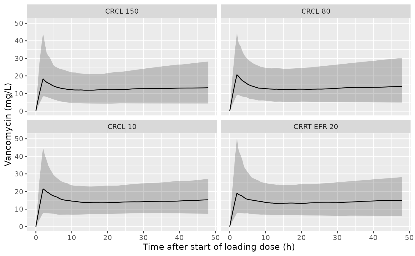
Simulated vancomycin concentrations over the first 48 h (median and 5th-95th percentile band) for four of the Table 3 strata.
PKNCA: AUC on day 2
conc <- sim |>
  dplyr::filter(!is.na(Cc)) |>
  dplyr::mutate(Cc = pmax(Cc, 0)) |>
  dplyr::select(id, time, Cc, stratum)
doses <- events |>
  dplyr::filter(evid == 1) |>
  dplyr::select(id, time, amt, stratum)

conc_obj <- PKNCA::PKNCAconc(conc, Cc ~ time | stratum + id)
dose_obj <- PKNCA::PKNCAdose(doses, amt ~ time | stratum + id)
intervals <- data.frame(start = 24, end = 48, auclast = TRUE)
nca <- PKNCA::pk.nca(PKNCA::PKNCAdata(conc_obj, dose_obj, intervals = intervals))

auc_ind <- as.data.frame(nca$result) |>
  dplyr::filter(PPTESTCD == "auclast") |>
  dplyr::select(stratum, id, auc = PPORRES)
stopifnot(nrow(auc_ind) == nrow(subjects), !anyNA(auc_ind$auc))

typ_conc <- sim_typ |>
  dplyr::filter(!is.na(Cc)) |>
  dplyr::select(id, time, Cc, stratum)
typ_nca <- PKNCA::pk.nca(PKNCA::PKNCAdata(
  PKNCA::PKNCAconc(typ_conc, Cc ~ time | stratum + id),
  PKNCA::PKNCAdose(
    make_events(typ_subj) |> dplyr::filter(evid == 1) |> dplyr::select(id, time, amt, stratum),
    amt ~ time | stratum + id
  ),
  intervals = intervals
))
auc_typ <- as.data.frame(typ_nca$result) |>
  dplyr::filter(PPTESTCD == "auclast") |>
  dplyr::select(stratum, auc_typ = PPORRES)
stopifnot(nrow(auc_typ) == 17L)
Comparison against the published dosing simulations
Table 3 reports the median AUC24-48 of the simulated
patients in each stratum, with a 95% interval, and the proportions
reaching AUC24-48 > 400, 400-600 and > 600
mg.h/L.
ref_wide <- tab3 |>
  dplyr::select(stratum, auclast = auc_pub)
cmp <- nlmixr2lib::ncaComparisonTable(
  simulated = auc_ind |> dplyr::mutate(PPTESTCD = "auclast", PPORRES = auc),
  reference = ref_wide,
  by = "stratum",
  params = "auclast",
  units = c(auclast = "mg*h/L")
)
knitr::kable(cmp, caption = "Median simulated AUC24-48 versus Table 3 of Garreau 2021.")| NCA parameter | stratum | Reference | Simulated | % diff |
|---|---|---|---|---|
| AUClast (mg*h/L) | CRCL 150 | 493 | 309 | -37.3%* |
| AUClast (mg*h/L) | CRCL 140 | 506 | 346 | -31.6%* |
| AUClast (mg*h/L) | CRCL 130 | 483 | 306 | -36.7%* |
| AUClast (mg*h/L) | CRCL 120 | 499 | 315 | -36.9%* |
| AUClast (mg*h/L) | CRCL 110 | 475 | 322 | -32.3%* |
| AUClast (mg*h/L) | CRCL 100 | 492 | 324 | -34.0%* |
| AUClast (mg*h/L) | CRCL 90 | 508 | 346 | -31.8%* |
| AUClast (mg*h/L) | CRCL 80 | 484 | 324 | -33.1%* |
| AUClast (mg*h/L) | CRCL 70 | 503 | 359 | -28.7%* |
| AUClast (mg*h/L) | CRCL 60 | 486 | 342 | -29.6%* |
| AUClast (mg*h/L) | CRCL 50 | 506 | 354 | -30.0%* |
| AUClast (mg*h/L) | CRCL 40 | 472 | 343 | -27.3%* |
| AUClast (mg*h/L) | CRCL 30 | 498 | 351 | -29.6%* |
| AUClast (mg*h/L) | CRCL 20 | 480 | 328 | -31.6%* |
| AUClast (mg*h/L) | CRCL 10 | 470 | 348 | -26.0%* |
| AUClast (mg*h/L) | CRRT EFR 30 | 494 | 316 | -36.1%* |
| AUClast (mg*h/L) | CRRT EFR 20 | 480 | 342 | -28.8%* |
sim_summary <- auc_ind |>
  dplyr::group_by(stratum) |>
  dplyr::summarise(
    median = median(auc),
    q025 = quantile(auc, 0.025), q975 = quantile(auc, 0.975),
    p400 = mean(auc > 400), pband = mean(auc > 400 & auc < 600), p600 = mean(auc > 600),
    .groups = "drop"
  ) |>
  dplyr::left_join(auc_typ, by = "stratum") |>
  dplyr::left_join(tab3, by = "stratum")

knitr::kable(
  sim_summary |>
    dplyr::transmute(
      stratum,
      md,
      pub = sprintf("%d [%d-%d]", auc_pub, auc_lo, auc_hi),
      sim = sprintf("%.0f [%.0f-%.0f]", median, q025, q975),
      typ = round(auc_typ),
      pta = sprintf("%.2f / %.2f / %.2f", pta400, pta_band, pta600),
      pta_sim = sprintf("%.2f / %.2f / %.2f", p400, pband, p600)
    ) |>
    dplyr::rename(
      Stratum = stratum,
      `Maintenance (mg/kg IBW/24 h)` = md,
      `Published AUC24-48 median [95%]` = pub,
      `Simulated median [95%]` = sim,
      `Typical value` = typ,
      `Published PTA >400 / 400-600 / >600` = pta,
      `Simulated PTA >400 / 400-600 / >600` = pta_sim
    ),
  caption = "Replicates Table 3 of Garreau 2021 (AUC in mg.h/L)."
)| Stratum | Maintenance (mg/kg IBW/24 h) | Published AUC24-48 median [95%] | Simulated median [95%] | Typical value | Published PTA >400 / 400-600 / >600 | Simulated PTA >400 / 400-600 / >600 |
|---|---|---|---|---|---|---|
| CRCL 150 | 30.0 | 493 [330-644] | 309 [75-687] | 332 | 0.80 / 0.64 / 0.16 | 0.28 / 0.21 / 0.07 |
| CRCL 140 | 30.0 | 506 [335-666] | 346 [118-796] | 348 | 0.83 / 0.62 / 0.21 | 0.39 / 0.30 / 0.09 |
| CRCL 130 | 27.5 | 483 [316-643] | 306 [69-715] | 341 | 0.77 / 0.63 / 0.14 | 0.29 / 0.23 / 0.07 |
| CRCL 120 | 27.5 | 499 [324-668] | 315 [103-712] | 358 | 0.80 / 0.61 / 0.19 | 0.36 / 0.29 / 0.07 |
| CRCL 110 | 25.0 | 475 [303-646] | 322 [86-699] | 350 | 0.74 / 0.60 / 0.14 | 0.32 / 0.27 / 0.05 |
| CRCL 100 | 25.0 | 492 [313-674] | 324 [92-799] | 367 | 0.77 / 0.58 / 0.19 | 0.34 / 0.22 / 0.12 |
| CRCL 90 | 25.0 | 508 [320-704] | 346 [81-836] | 385 | 0.80 / 0.55 / 0.25 | 0.38 / 0.29 / 0.08 |
| CRCL 80 | 22.5 | 484 [298-684] | 324 [94-718] | 376 | 0.75 / 0.56 / 0.19 | 0.32 / 0.23 / 0.09 |
| CRCL 70 | 22.5 | 503 [307-720] | 359 [114-769] | 395 | 0.78 / 0.55 / 0.23 | 0.35 / 0.26 / 0.10 |
| CRCL 60 | 20.0 | 486 [287-706] | 342 [119-762] | 384 | 0.74 / 0.53 / 0.21 | 0.35 / 0.27 / 0.09 |
| CRCL 50 | 20.0 | 506 [295-751] | 354 [128-845] | 404 | 0.77 / 0.50 / 0.27 | 0.41 / 0.29 / 0.12 |
| CRCL 40 | 17.5 | 472 [273-707] | 343 [151-679] | 393 | 0.69 / 0.50 / 0.19 | 0.41 / 0.33 / 0.08 |
| CRCL 30 | 17.5 | 498 [283-761] | 351 [121-783] | 415 | 0.74 / 0.47 / 0.27 | 0.38 / 0.25 / 0.12 |
| CRCL 20 | 15.0 | 480 [265-767] | 328 [146-682] | 403 | 0.69 / 0.44 / 0.25 | 0.31 / 0.26 / 0.06 |
| CRCL 10 | 12.5 | 470 [245-776] | 348 [156-644] | 394 | 0.66 / 0.42 / 0.24 | 0.36 / 0.30 / 0.06 |
| CRRT EFR 30 | 20.0 | 494 [295-723] | 316 [115-695] | 361 | 0.74 / 0.50 / 0.24 | 0.32 / 0.26 / 0.06 |
| CRRT EFR 20 | 17.5 | 480 [277-728] | 342 [108-708] | 390 | 0.71 / 0.49 / 0.22 | 0.34 / 0.27 / 0.07 |
The model does not reproduce Table 3 numerically, and the mismatch has two separate parts.
-
Level. The typical-value
AUC24-48runs about 15-35% below the published medians, and the medians of the simulated cohort sit lower still, because of the large clearance variability discussed next. The shortfall is largest in the high-CRCL strata, where the exponential covariate term raises clearance most steeply. No reading of the printed parameters closes the gap. The plain power form of Eq. (1) overshoots instead, by roughly 45-70% for the same regimens, and it is excluded independently by the Figure 1 prediction range (see above). -
Spread. The published 95% intervals, for example
330-644 mg.h/L at CRCL 150, correspond to a log-scale SD of
AUC24-48of about 0.17-0.25. The Table 2 random effects are much larger.omega_CL= 0.76 alone would carry through almost in full to a steady-state AUC. The simulated day-2 intervals above correspond to a log-scale SD of about 0.35-0.55, so they are several-fold wider than the published ones, and the simulated proportion in the 400-600 band is correspondingly lower. The paper’s own pcVPC (Figure 2) also shows simulated 10th-90th percentile bands of only about 20-38 mg/L at steady state, which is again narrower thanomega_CL= 0.76 implies. The Table 2 values are transcribed as printed (labelled “standard deviation”). The paper gives no information that would reconcile its Simulx runs with them.
The structural check that does hold is the dose selection itself. The
paper chose each stratum’s maintenance dose so that the median
AUC24-48 sits near the 400-600 centre, which makes Table 3
flat (470-508) across a 2.4-fold dose range. The model’s typical-value
AUCs for the same doses are also flat to within about +/- 12%. The gate
below guards that flatness and records the level offset as a band. The
band excludes a clearance or volume mis-transcription of more than about
15%.
chk <- sim_summary |>
  dplyr::mutate(ratio_typ = auc_typ / auc_pub)
stopifnot(nrow(chk) == 17L, !anyNA(chk$ratio_typ))
# Deterministic (typical-value) quantities, so the bounds do not depend on the
# simulated cohort. Measured: ratio 0.67-0.84 across the 17 strata, median 0.78;
# typical-value AUC range 332-415 mg.h/L.
stopifnot(
  all(chk$ratio_typ > 0.60), all(chk$ratio_typ < 0.92),
  abs(median(chk$ratio_typ) - 0.78) < 0.06,
  max(chk$auc_typ) / min(chk$auc_typ) < 1.35
)
Replication of Figure 2 (learning-set concentrations)
Figure 2 is a prediction-corrected VPC of the learning data out to about 160 h. The observed percentiles, read from the figure, are about 21 mg/L (median) at 12 h and 25-26 mg/L from 40 h onward. The 10th percentile is 15 mg/L at 12 h and 19-20 mg/L thereafter, and the 90th percentile is 33-40 mg/L. The chunk below simulates a cohort that resembles the learning set on the paper’s mean regimen. It gives a loading dose of 22.7 mg/kg over 2 h and then 28.6 mg/kg/day by continuous infusion, both assumed to be per kg of total body weight. 28% of the cohort is on CRRT.
n_fig2 <- 200L
set.seed(2013)
fig2_subj <- tibble::tibble(
  id = seq_len(n_fig2),
  RRT_CRRT_STATUS = as.numeric(seq_len(n_fig2) <= round(0.282 * n_fig2)),
  WT = draw_trunc(n_fig2, 77.9, 20.4, 45, 140),
  IBW = draw_trunc(n_fig2, 63.5, 9, 45, 85),
  crcl_draw = draw_trunc(n_fig2, 50.4, 29, 10, 150),
  efr_draw = draw_trunc(n_fig2, 35.6, 18.7, 15, 80)
) |>
  dplyr::mutate(
    CRCL = ifelse(RRT_CRRT_STATUS == 1, 0, crcl_draw),
    RRT_CRRT_EFFLUENT_FLOW = ifelse(RRT_CRRT_STATUS == 1, efr_draw * 60, 0)
  )
fig2_times <- c(0, seq(2, 160, by = 2))
fig2_ev <- dplyr::bind_rows(
  fig2_subj |> dplyr::mutate(time = 0, amt = 22.7 * WT, rate = 22.7 * WT / 2, evid = 1),
  fig2_subj |> dplyr::mutate(time = 2, rate = 28.6 * WT / 24, amt = 28.6 * WT / 24 * 158, evid = 1),
  fig2_subj |>
    dplyr::slice(rep(seq_len(n_fig2), each = length(fig2_times))) |>
    dplyr::mutate(time = rep(fig2_times, times = n_fig2), amt = 0, rate = 0, evid = 0)
) |>
  dplyr::mutate(cmt = "central") |>
  dplyr::arrange(id, time, dplyr::desc(evid)) |>
  dplyr::select(id, time, amt, rate, evid, cmt, CRCL, IBW, RRT_CRRT_STATUS, RRT_CRRT_EFFLUENT_FLOW)

fig2_sim <- rxode2::rxSolve(mod, events = fig2_ev, maxsteps = 1e6, returnType = "data.frame")
fig2_q <- fig2_sim |>
  dplyr::filter(!is.na(sim), time >= 2) |>
  dplyr::group_by(time) |>
  dplyr::summarise(
    p10 = quantile(sim, 0.10), p50 = median(sim), p90 = quantile(sim, 0.90),
    .groups = "drop"
  ) |>
  tidyr::pivot_longer(-time, names_to = "percentile", values_to = "conc")

fig2_obs <- tibble::tribble(
  ~time, ~p10, ~p50, ~p90,
  12,    15,   21,   33,
  40,    20,   25,   37,
  60,    20,   26,   40,
  90,    20,   25,   36,
  140,   19,   25,   33
) |>
  tidyr::pivot_longer(-time, names_to = "percentile", values_to = "conc")

ggplot(fig2_q, aes(time, conc, colour = percentile)) +
  geom_line() +
  geom_point(data = fig2_obs, size = 2) +
  labs(
    x = "Time after first dose (h)", y = "Vancomycin (mg/L)",
    colour = "Percentile"
  )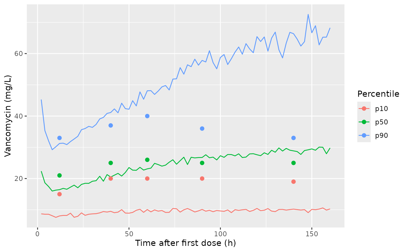
Simulated 10th, 50th and 90th percentiles for a learning-set-like cohort on the mean Table 1 regimen (lines), with the approximate observed percentiles of Figure 2 of Garreau 2021 (points).
fig2_cmp <- fig2_obs |>
  dplyr::rename(observed = conc) |>
  dplyr::left_join(fig2_q |> dplyr::rename(simulated = conc), by = c("time", "percentile"))
stopifnot(nrow(fig2_cmp) == 15L, !anyNA(fig2_cmp$simulated))
knitr::kable(
  fig2_cmp |>
    dplyr::mutate(simulated = round(simulated, 1)) |>
    tidyr::pivot_wider(names_from = percentile, values_from = c(observed, simulated)) |>
    dplyr::rename(
      `Time (h)` = time,
      `Observed P10` = observed_p10, `Observed P50` = observed_p50, `Observed P90` = observed_p90,
      `Simulated P10` = simulated_p10, `Simulated P50` = simulated_p50, `Simulated P90` = simulated_p90
    ),
  caption = "Approximate observed percentiles of Figure 2 versus the simulated cohort (mg/L)."
)| Time (h) | Observed P10 | Observed P50 | Observed P90 | Simulated P10 | Simulated P50 | Simulated P90 |
|---|---|---|---|---|---|---|
| 12 | 15 | 21 | 33 | 8.0 | 16.4 | 31.2 |
| 40 | 20 | 25 | 37 | 9.5 | 20.5 | 41.1 |
| 60 | 20 | 26 | 40 | 10.1 | 23.1 | 48.1 |
| 90 | 20 | 25 | 36 | 10.1 | 26.7 | 57.8 |
| 140 | 19 | 25 | 33 | 10.2 | 28.9 | 66.4 |
The simulated median stays within about 25% of the observed median at each time read from the figure: 16 versus 21 mg/L at 12 h, and 29 versus 25 mg/L at 140 h. It keeps rising after 90 h, while the observed median is flat. The simulated 10th-90th band is much wider than the observed one, about 10-66 mg/L against 19-33 mg/L at 140 h. That is the spread discrepancy discussed under Table 3. Therapeutic drug monitoring narrows the observed band further and flattens its late median: each patient’s infusion rate was adjusted to the measured concentrations, while the simulation holds the mean regimen fixed. The figure is shown for orientation and is not gated.
Assumptions and deviations
- Covariate form. The exponential-of-power form printed with Table 2 is used in preference to the plain power form of Methods Eq. (1). The reasons are given above, and the plain power form is excluded by the Figure 1 prediction range.
-
Covariate exponents 0.5 (CRCL) and 0.69 (CRRT effluent
flow) appear only in the Table 2 final-model equations. They
are absent from the Table 2 list of estimated fixed effects, which does
include the IBW exponent
alphawith its RSE. They are encoded withfixed()on that basis. The paper does not say explicitly whether they were fixed or estimated. - V2. Table 2 prints 61.3 L and the Sect. 2.2 prose prints 63.1 L. The table value is used.
-
Discussion values. The Discussion quotes a “typical
V1 of 0.43 L/kg (TBW)”. That figure equals
V1pop / mean IBW = 27.3 / 63.5(IBW, not TBW), and it does not include thee^((IBW/64.1)^alpha)factor. The accompanying “typical CL of 0.0185 L/h/kg” is not reproduced by any combination of printed values. Neither statement is used. - CRRT effluent flow units. The paper reports mL/min and centres at 20 mL/min. The canonical column is mL/h, so the model divides by 1200 mL/h.
-
CRRT as a subject-level flag. CRRT is encoded as
RRT_CRRT_STATUS. CRCL is 0 in CRRT patients by the paper’s convention, and the effluent flow is ignored off CRRT. - Table 3 simulations. The IBW distribution of the paper’s virtual patients is not reported. It was drawn here from the learning-set summary. The maintenance infusion is assumed to start when the 2-h loading infusion ends; the paper does not say whether it overlapped the loading infusion.
- Figure 2 replication. The dose-per-kg basis of the Table 1 mean regimen is not stated, and total body weight was assumed. The observed percentiles were read by eye from the figure.
-
Not reproduced. Neither the level nor the spread of
the published
AUC24-48distribution in Tables 3-4 is reproduced; see the discussion under “Comparison against the published dosing simulations”. The model is transcribed as printed, without adjustment.