Tacrolimus starting dose in paediatric renal transplant recipients (Andrews 2020)
Source:vignettes/articles/Andrews_2020_tacrolimus.Rmd
Andrews_2020_tacrolimus.RmdThe paper
Andrews LM, de Winter BCM, Cornelissen EAM, de Jong H, Hesselink DA, Schreuder MF, Bruggemann RJM, van Gelder T, Cransberg K. A Population Pharmacokinetic Model Does Not Predict the Optimal Starting Dose of Tacrolimus in Pediatric Renal Transplant Recipients in a Prospective Study: Lessons Learned and Model Improvement. Clin Pharmacokinet. 2020;59(5):591-603. doi:10.1007/s40262-019-00831-8
The paper has two parts. First, a prospective trial dosed 16 children
with the starting-dose algorithm of the earlier Andrews 2017 model
(available here as modellib("Andrews_2017_tacrolimus"));
only 31% reached the target pre-dose concentration (C0) on day 3, and
the trial was stopped. Second, the model was re-fitted on an expanded
cohort of 95 children, giving:
- a final model (Equation 2) with CYP3A5 genotype, haematocrit and serum creatinine on CL/F, and
- a starting-dose model (Equation 3) with only the pre-transplant covariates – bodyweight and CYP3A5 genotype – which defines the improved dosing algorithm (Equation 4).
Both are distributed here and both are exercised below. The base model in Table 4 is not distributed.
mod_final <- modellib("Andrews_2020_tacrolimus")
mod_start <- modellib("Andrews_2020_tacrolimus_startingdose")
rx_final <- rxode2::rxode2(mod_final)
#> ℹ parameter labels from comments will be replaced by 'label()'
rx_start <- rxode2::rxode2(mod_start)
#> ℹ parameter labels from comments will be replaced by 'label()'
rx_final$state
#> [1] "depot"       "central"     "peripheral1"
Population
The model-building cohort (Table 3) had 95 paediatric kidney transplant recipients from Erasmus MC-Sophia Children’s Hospital (Rotterdam) and Radboudumc Amalia Children’s Hospital (Nijmegen): 61% male, median age 11.4 years (1.6-17.9), median bodyweight 32.0 kg (10.4-87.5), median haematocrit 0.29 L/L (0.16-0.52) and median creatinine 84 umol/L (12-1454). CYP3A5 genotype was 1/1 in 3, 1/3 in 11, 3/3 in 52, 3/7 in 2 and unknown in 27 children. 78% received a living-donor kidney. All received twice-daily immediate-release tacrolimus (capsules or granules) with basiliximab, mycophenolic acid and a 5-day glucocorticoid course. The 1338 whole-blood samples were collected over the first 42 days post-transplant; 95.2% were measured by LC-MS/MS and 4.8% by immunoassay.
Source trace
| Quantity | Value | Source |
|---|---|---|
| Structure (2-cmt, first-order absorption, lag) | 2-cmt | Results 3.2.1 |
| tlag | 0.41 h (held constant) | Table 4 ‘t lag (h) FIX’ |
| ka, CL/F, V1/F, Q/F, V2/F (final) | 1.7 1/h, 36.6 L/h, 496 L, 31.7 L/h, 1270 L | Table 4, final model |
| ka, CL/F, V1/F, Q/F, V2/F (starting dose) | 1.85 1/h, 34.5 L/h, 540 L, 28.5 L/h, 1660 L | Table 4, starting dose model |
| Weight exponent on CL/F | 0.62 (final), 0.56 (starting dose) | Table 4; Equations (2), (3) |
| Weight exponent on V1/F, V2/F | 1 (held constant) | Results 3.2.1 |
| Q/F, ka weight scaling | none | Table 4 units (‘L/h’, not ‘L/h/70 kg’) |
| CYP3A5 expresser factor | 1.4 (final), 1.46 (starting dose) | Equations (2), (3); Table 4 rounds 1.46 to 1.5 |
| Haematocrit effect | (HCT/0.29)^-0.60 | Equation (2); Table 4 |
| Creatinine effect | (CREAT/84)^-0.1 | Equation (2); Table 4 |
| IIV (CV%) ka, CL/F, V1/F, V2/F (final) | 183, 42.1, 99.6, 85.2 | Table 4 |
| IIV (CV%) ka, CL/F, V1/F, V2/F (starting dose) | 178, 42.3, 93.0, 89.3 | Table 4 |
| IOV on CL/F | 20.1% | Table 4 (not encoded; see Assumptions) |
| Residual error, final (add ng/mL; prop) | IA 1.27, 0.11; LC-MS/MS 0.87, 0.23 | Table 4 |
| Residual error, starting dose (add ng/mL; prop) | IA 1.01, 0.12; LC-MS/MS 0.96, 0.24 | Table 4 |
| C0 to AUC0-12h mapping | 10 -> 185; 12.5 -> 220; 15 -> 254 ng*h/mL | Results 3.2.1 |
| Improved dosing algorithm | 220 * CL/F / 1000 | Equation (4) |
| Example doses | mg/kg/day by weight and CYP3A5 | ESM Table S3 |
Structural check: the closed-form AUC identity
For a linear model, the single-dose AUC to infinity equals
Dose / (CL/F). Both sides use the same parameters, so the
check is tight.
grid_long <- sort(unique(c(
  seq(0, 24, by = 0.25), seq(24, 240, by = 2), seq(240, 24 * 60, by = 12)
)))
d_single <- as.data.frame(
  rxode2::et(amt = 5, cmt = "depot") |> rxode2::et(grid_long, cmt = "central")
)
d_single$WT <- 70
d_single$HCT <- 29
d_single$CREAT <- 84
d_single$CYP3A5_EXPR <- 0
d_single$IMMUNOASSAY <- 0

sim_single <- rxode2::rxSolve(
  rx_final, d_single, omega = NA, sigma = NA, returnType = "data.frame"
) |>
  dplyr::filter(!is.na(Cc))

trapz <- function(x, y) sum(diff(x) * (utils::head(y, -1) + utils::tail(y, -1)) / 2)
auc_sim <- trapz(sim_single$time, sim_single$Cc)
auc_cf <- 5 / 36.6 * 1000
c(simulated = auc_sim, closed_form = auc_cf, pct_diff = 100 * (auc_sim - auc_cf) / auc_cf)
#>    simulated  closed_form     pct_diff
#> 136.67279018 136.61202186 0.04448241Covariate effects: reproducing the paper’s numbers
Section 3.2.3 states three quantitative covariate effects on CL/F for
the final model. The paper expresses the haematocrit and creatinine
effects as the fractional reduction of CL/F at the higher
covariate value (1 - CL(high) / CL(low)); read that way,
the exponents reproduce the printed percentages.
e <- function(model, nm) {
  ini <- as.data.frame(rxode2::rxode2(model)$iniDf)
  ini$est[match(nm, ini$name)]
}
claims <- tibble::tribble(
  ~Claim, ~Paper, ~Model,
  "CYP3A5 expressers: fold higher CL/F", 1.4, e(mod_final, "e_cyp3a5_expr_cl"),
  "Haematocrit 0.35 vs 0.25 L/L: % CL/F difference", 18,
  100 * (1 - (0.35 / 0.25)^e(mod_final, "e_hct_cl")),
  "Creatinine 500 vs 50 umol/L: % CL/F difference", 21,
  100 * (1 - (500 / 50)^e(mod_final, "e_creat_cl"))
) |>
  dplyr::mutate(`% diff` = 100 * (Model - Paper) / Paper)
#> ℹ parameter labels from comments will be replaced by 'label()'
#> ℹ parameter labels from comments will be replaced by 'label()'
#> ℹ parameter labels from comments will be replaced by 'label()'
knitr::kable(claims, digits = 2)| Claim | Paper | Model | % diff |
|---|---|---|---|
| CYP3A5 expressers: fold higher CL/F | 1.4 | 1.40 | 0.00 |
| Haematocrit 0.35 vs 0.25 L/L: % CL/F difference | 18.0 | 18.28 | 1.56 |
| Creatinine 500 vs 50 umol/L: % CL/F difference | 21.0 | 20.57 | -2.06 |
# The paper rounds to two significant figures (exact: 18.28% and 20.57%);
# a wrong-signed or mis-transcribed exponent moves these by tens of percent.
stopifnot(max(abs(claims$`% diff`)) < 3)
Covariate profiles (cf. ESM Figure S2)
Typical-value steady-state profiles over one dosing interval for a 32 kg child (the cohort median) on 0.15 mg/kg twice daily, varying one covariate at a time with the others held at their centring values.
profile_for <- function(cov, label) {
  ev <- rxode2::et(amt = 0.15 * cov$WT, ii = 12, until = 24 * 28, cmt = "depot") |>
    rxode2::et(seq(24 * 28, 24 * 28 + 12, by = 0.25), cmt = "central")
  d <- as.data.frame(ev)
  for (nm in names(cov)) d[[nm]] <- cov[[nm]]
  rxode2::rxSolve(rx_final, d, omega = NA, sigma = NA, returnType = "data.frame") |>
    dplyr::filter(!is.na(Cc)) |>
    dplyr::mutate(time = time - 24 * 28, level = label)
}
ref <- list(WT = 32, HCT = 29, CREAT = 84, CYP3A5_EXPR = 0, IMMUNOASSAY = 0)
with_cov <- function(nm, v) {
  x <- ref
  x[[nm]] <- v
  x
}
panels <- dplyr::bind_rows(
  dplyr::bind_rows(lapply(c(0, 1), function(v) {
    profile_for(with_cov("CYP3A5_EXPR", v), c("non-expresser", "expresser")[v + 1])
  })) |> dplyr::mutate(panel = "A: CYP3A5"),
  dplyr::bind_rows(lapply(c(15, 32, 60), function(v) {
    profile_for(with_cov("WT", v), paste(v, "kg"))
  })) |> dplyr::mutate(panel = "B: bodyweight"),
  dplyr::bind_rows(lapply(c(50, 100, 500), function(v) {
    profile_for(with_cov("CREAT", v), paste(v, "umol/L"))
  })) |> dplyr::mutate(panel = "C: creatinine"),
  dplyr::bind_rows(lapply(c(25, 30, 35), function(v) {
    profile_for(with_cov("HCT", v), paste0(v, "%"))
  })) |> dplyr::mutate(panel = "D: haematocrit")
)
ggplot(panels, aes(time, Cc, colour = level)) +
  geom_line() +
  facet_wrap(~panel, ncol = 2) +
  labs(x = "Time after dose (h)", y = "Tacrolimus (ng/mL)", colour = NULL,
       title = "Typical-value steady-state profiles, final model") +
  theme_bw(base_size = 9)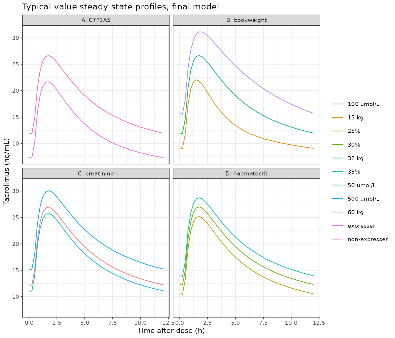
The improved dosing algorithm (Equation 4, ESM Table S3)
Equation (4) is Dose = 220 * CL/F / 1000 with the
starting-dose model’s CL/F. Because AUC0-12h times CL/F is the amount
given per 12-h interval, the equation gives the dose per administration;
the daily dose is twice that. The ESM Table S3 example doses (mg/kg/day)
confirm this reading: for a 70 kg non-expresser,
2 * 220 * 34.5 / 1000 / 70 = 0.217 against 0.22 in Table
S3.
cl_start <- function(wt, cyp) {
  exp(e(mod_start, "lcl")) * (wt / 70)^e(mod_start, "e_wt_cl") *
    (1 + (e(mod_start, "e_cyp3a5_expr_cl") - 1) * cyp)
}
dose_q12h <- function(wt, cyp) 220 * cl_start(wt, cyp) / 1000

s3 <- tibble::tibble(
  WT = rep(seq(10, 80, by = 10), 2),
  CYP3A5_EXPR = rep(c(1, 0), each = 8),
  table_s3 = c(0.73, 0.54, 0.46, 0.40, 0.37, 0.34, 0.32, 0.30,
               0.50, 0.37, 0.31, 0.28, 0.25, 0.23, 0.22, 0.20)
) |>
  dplyr::mutate(
    model = 2 * dose_q12h(WT, CYP3A5_EXPR) / WT,
    pct_diff = 100 * (model - table_s3) / table_s3
  )
#> ℹ parameter labels from comments will be replaced by 'label()'
#> ℹ parameter labels from comments will be replaced by 'label()'
#> ℹ parameter labels from comments will be replaced by 'label()'
s3 |>
  dplyr::mutate(CYP3A5_EXPR = ifelse(CYP3A5_EXPR == 1, "expresser", "non-expresser")) |>
  dplyr::rename(
    "Weight (kg)" = WT, "CYP3A5" = CYP3A5_EXPR,
    "Table S3 (mg/kg/day)" = table_s3, "Model (mg/kg/day)" = model, "% diff" = pct_diff
  ) |>
knitr::kable(digits = 3)| Weight (kg) | CYP3A5 | Table S3 (mg/kg/day) | Model (mg/kg/day) | % diff |
|---|---|---|---|---|
| 10 | expresser | 0.73 | 0.745 | 2.105 |
| 20 | expresser | 0.54 | 0.549 | 1.747 |
| 30 | expresser | 0.46 | 0.460 | -0.074 |
| 40 | expresser | 0.40 | 0.405 | 1.252 |
| 50 | expresser | 0.37 | 0.367 | -0.775 |
| 60 | expresser | 0.34 | 0.339 | -0.344 |
| 70 | expresser | 0.32 | 0.317 | -1.059 |
| 80 | expresser | 0.30 | 0.299 | -0.485 |
| 10 | non-expresser | 0.50 | 0.511 | 2.105 |
| 20 | non-expresser | 0.37 | 0.376 | 1.710 |
| 30 | non-expresser | 0.31 | 0.315 | 1.560 |
| 40 | non-expresser | 0.28 | 0.277 | -0.928 |
| 50 | non-expresser | 0.25 | 0.251 | 0.584 |
| 60 | non-expresser | 0.23 | 0.232 | 0.903 |
| 70 | non-expresser | 0.22 | 0.217 | -1.429 |
| 80 | non-expresser | 0.20 | 0.204 | 2.242 |
# Table S3 is printed to two decimals, so rounding alone is up to about 2.5%
# at the lowest doses. A missing factor of 2 (per-dose vs daily) or a wrong
# exponent or CYP3A5 factor fails this by far more.
stopifnot(max(abs(s3$pct_diff)) < 3.5)
The model runs about 2% above Table S3 at 10-20 kg and within about 1% at 50-80 kg; the low-weight rows would be reproduced exactly by a weight exponent of about 0.57, so the table was probably generated from the unrounded estimate rather than the printed 0.56.
Virtual cohort and steady-state exposure under Equation 4
The purpose of the starting-dose model is to set a dose that achieves the C0 target of 12.5 ng/mL, which the paper maps to an AUC0-12h of 220 ngh/mL. Dosing a virtual cohort by Equation (4) and computing AUC0-12h with PKNCA at steady state checks that the model and the algorithm agree: with log-normal IIV on CL/F, the median* AUC should sit at the target.
Bodyweight is drawn log-normally around the cohort median (32 kg), truncated to the observed 10.4-87.5 kg range. The two arms are CYP3A5 non-expressers and expressers (100 children each). All samples are LC-MS/MS.
rxode2::rxSetSeed(20191026)
set.seed(20191026)
n_per_arm <- 100L
cohort <- tibble::tibble(
  id = seq_len(2 * n_per_arm),
  CYP3A5_EXPR = rep(c(0, 1), each = n_per_arm),
  arm = rep(c("non-expresser", "expresser"), each = n_per_arm),
  WT = pmin(pmax(rlnorm(2 * n_per_arm, log(32), 0.55), 10.4), 87.5),
  IMMUNOASSAY = 0
) |>
  dplyr::mutate(dose = dose_q12h(WT, CYP3A5_EXPR))
#> ℹ parameter labels from comments will be replaced by 'label()'
#> ℹ parameter labels from comments will be replaced by 'label()'
#> ℹ parameter labels from comments will be replaced by 'label()'
summary(cohort$WT)
#>    Min. 1st Qu.  Median    Mean 3rd Qu.    Max.
#>   10.40   21.21   29.93   35.61   46.85   87.50
tau <- 12
t_ss <- 24 * 28
ev <- do.call(rbind, lapply(seq_len(nrow(cohort)), function(i) {
  rbind(
    data.frame(id = cohort$id[i], time = seq(0, t_ss, by = tau),
               amt = cohort$dose[i], evid = 1L, cmt = "depot"),
    data.frame(id = cohort$id[i], time = t_ss + c(0, 0.5, 1, 1.5, 2, 3, 4, 6, 8, 10, 12),
               amt = NA_real_, evid = 0L, cmt = "central")
  )
}))
ev <- merge(ev, cohort[, c("id", "WT", "CYP3A5_EXPR", "IMMUNOASSAY", "arm")], by = "id")
ev <- ev[order(ev$id, ev$time, -ev$evid), ]

sim <- rxode2::rxSolve(rx_start, ev, keep = "arm", returnType = "data.frame")

sim_ss <- sim |>
  dplyr::filter(time >= t_ss) |>
  dplyr::mutate(time = time - t_ss)

ggplot(sim_ss, aes(time, Cc, group = id)) +
  geom_line(alpha = 0.15) +
  stat_summary(aes(group = NULL), fun = median, geom = "line", colour = "red", linewidth = 1) +
  geom_hline(yintercept = 12.5, linetype = 2) +
  facet_wrap(~arm) +
  scale_y_log10() +
  labs(x = "Time after dose (h)", y = "Tacrolimus (ng/mL)",
       title = "Steady-state profiles under Equation 4 dosing (day 28)",
       subtitle = "Red: median; dashed: 12.5 ng/mL C0 target") +
  theme_bw()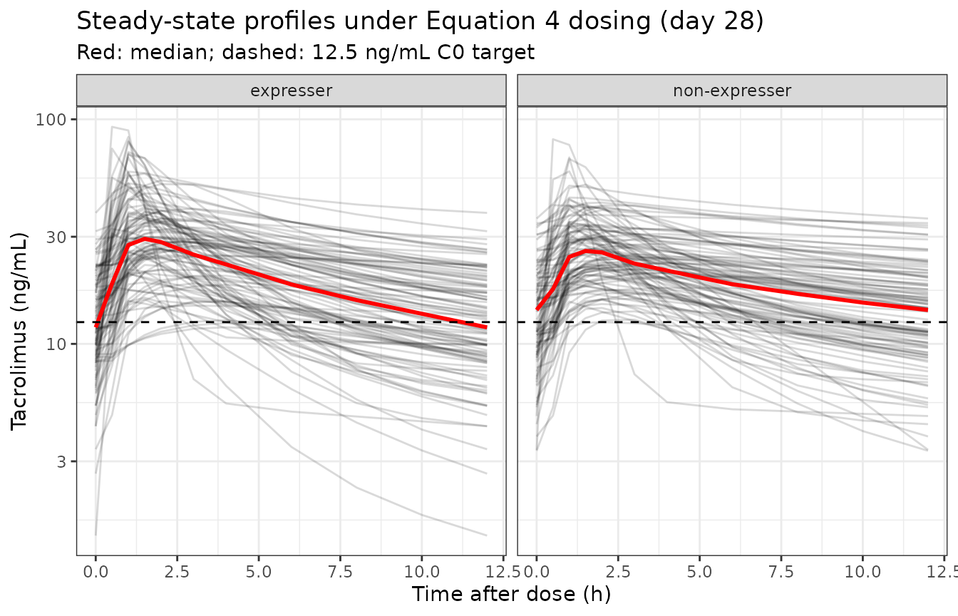
conc <- sim_ss |>
  dplyr::filter(!is.na(Cc)) |>
  dplyr::select(id, time, Cc, arm)
doses <- cohort |>
  dplyr::transmute(id, time = 0, dose, arm)

conc_obj <- PKNCA::PKNCAconc(conc, Cc ~ time | arm + id)
dose_obj <- PKNCA::PKNCAdose(doses, dose ~ time | arm + id)
intervals <- data.frame(start = 0, end = 12, auclast = TRUE, cmax = TRUE,
                        tmax = TRUE, ctrough = TRUE)
nca <- PKNCA::pk.nca(PKNCA::PKNCAdata(conc_obj, dose_obj, intervals = intervals))
nca_res <- as.data.frame(nca$result)

nca_sum <- nca_res |>
  dplyr::group_by(arm, PPTESTCD) |>
  dplyr::summarise(median = median(PPORRES), .groups = "drop") |>
  tidyr::pivot_wider(names_from = PPTESTCD, values_from = median)
nca_sum |>
  dplyr::rename("Arm" = arm, "AUC0-12 (ng*h/mL)" = auclast, "Cmax (ng/mL)" = cmax,
                "C0 (ng/mL)" = ctrough, "Tmax (h)" = tmax) |>
knitr::kable(digits = 2, caption = "Median steady-state NCA under Equation 4 dosing")| Arm | AUC0-12 (ng*h/mL) | Cmax (ng/mL) | C0 (ng/mL) | Tmax (h) |
|---|---|---|---|---|
| expresser | 232.48 | 29.92 | 11.84 | 1.5 |
| non-expresser | 220.06 | 26.70 | 14.15 | 1.5 |
auc_chk <- nca_res |>
  dplyr::filter(PPTESTCD == "auclast") |>
  dplyr::mutate(pct_diff = 100 * (PPORRES - 220) / 220)

# Reference: the design target of Equation (4) (AUC0-12h 220 ng*h/mL) and the
# C0 of 12.5 ng/mL that Results 3.2.1 maps to it.
reference_nca <- tibble::tibble(
  arm = c("non-expresser", "expresser"),
  auclast = 220,
  ctrough = 12.5
)
cmp <- nlmixr2lib::ncaComparisonTable(
  nca_res |> dplyr::filter(PPTESTCD %in% c("auclast", "ctrough")),
  reference_nca,
  by = "arm",
  units = c(auclast = "ng*h/mL", ctrough = "ng/mL"),
  tolerance_pct = 20
)
knitr::kable(cmp)| NCA parameter | arm | Reference | Simulated | % diff |
|---|---|---|---|---|
| AUClast (ng*h/mL) | non-expresser | 220 | 220 | +0.0% |
| AUClast (ng*h/mL) | expresser | 220 | 232 | +5.7% |
| Ctrough (ng/mL) | non-expresser | 12.5 | 14.2 | +13.2% |
| Ctrough (ng/mL) | expresser | 12.5 | 11.8 | -5.3% |
attr(cmp, "footnote")
#> NULL
# Median AUC0-12 at the design target. With 42% CV on CL/F, the Monte Carlo
# standard error of a median is about 5% at n = 100 per arm and about 4% for
# the pooled 200, so the bounds are set near 3 standard errors. Tails are not
# asserted: they depend on which subjects the RNG draws. A mis-read dose basis
# (per-dose vs daily) would put the median 100% off.
med_by_arm <- tapply(auc_chk$pct_diff, auc_chk$arm, median)
med_by_arm
#>     expresser non-expresser
#>    5.67277616    0.02905356
stopifnot(
  abs(median(auc_chk$pct_diff)) < 10,
  all(abs(med_by_arm) < 15)
)
The median AUC0-12h lands on the 220 ng*h/mL design target in both
arms (the few-percent residual is Monte Carlo error at 100 children per
arm), confirming that Equation (4) is AUC * CL/F for the
starting-dose model. The simulated median C0 (Cmin) can be compared with
the 12.5 ng/mL target the paper maps to that AUC: the mapping in Results
3.2.1 was derived from the paper’s data, not from the typical-value
model, so it is reported here rather than asserted.
Assumptions and deviations
- Inter-occasion variability on CL/F (20.1% CV in both the final and starting-dose models) is not encoded. The paper does not define an occasion (it refers to the Andrews 2017 methods, which do not either); this matches the Andrews 2017 and Andrews 2019 tacrolimus models in the library. IOV would widen within-subject variability but not change typical values.
-
IIV scale. Table 4 reports IIV as %CV; variances
were computed as
log(1 + CV^2), the convention used for the sibling Andrews models. - Units typos. Table 4 labels ka in ‘L/h’; it is a first-order rate constant (1/h).
- Q/F and ka are not weight-scaled. Results 3.2.1 names allometric scaling on CL/F, V1/F and V2/F only, and Table 4 gives Q/F in ‘L/h’ where the scaled parameters are ‘per 70 kg’.
-
CYP3A5 unknown genotype. 28% of the cohort had no
genotype and the paper does not state how they were coded; users without
a genotype should set
CYP3A5_EXPR = 0(the Andrews 2017 convention). 3/7 is treated as a non-expresser. - CYP3A5 factor in the starting-dose model is taken as 1.46 from Equations (3) and (4) (Table 4 rounds it to 1.5).
- Haematocrit is on the canonical percent scale (centred at 29%), which is numerically identical to the paper’s 0.29 L/L centring.
- Equation 4 dose basis. As printed, Equation (4) is labelled mg/day but gives the dose per 12-h administration; the ESM Table S3 example doses confirm that the daily dose is twice the Equation (4) value.