Everolimus (Itohara 2022)
Source:vignettes/articles/Itohara_2022_everolimus.Rmd
Itohara_2022_everolimus.RmdModel and source
- Citation: Itohara K, Yano I, Nakagawa S, Sugimoto M, Hirai M, Yonezawa A, Imai S, Nakagawa T, Hira D, Ito T, Hata K, Hatano E, Terada T, Matsubara K. Population pharmacokinetics of everolimus in adult liver transplant patients: Comparison to tacrolimus disposition and extrapolation to pediatrics. Clin Transl Sci. 2022;15(11):2652-2662. doi:10.1111/cts.13389.
- Description (final model): One-compartment population PK model with first-order absorption for oral everolimus in Japanese adult liver transplant recipients (Itohara 2022 final model). Apparent oral clearance scales allometrically with body weight (fixed exponent 0.75) and carries power effects of the total daily everolimus dose (a therapeutic-drug-monitoring artefact, not nonlinearity) and of eGFR, plus multiplicative effects of concomitant fluconazole and female sex; the apparent volume scales linearly with body weight. The absorption rate constant is fixed from the literature. Everolimus is assayed in whole blood and concentrations are in ng/mL.
- Description (model with the prior tacrolimus D/C ratio): One-compartment population PK model with first-order absorption for oral everolimus in Japanese adult liver transplant recipients who were on tacrolimus before starting everolimus (Itohara 2022, model with the prior tacrolimus dose-per-trough ratio). Identical in form to Itohara_2022_everolimus (allometric body weight, total daily everolimus dose, eGFR, fluconazole and female sex on apparent clearance; body weight on the apparent volume) with an added power effect of the pre-everolimus tacrolimus dose-per-trough (D/C) ratio on apparent clearance, all parameters re-estimated. Everolimus is assayed in whole blood and concentrations are in ng/mL.
- Article (open access): https://doi.org/10.1111/cts.13389
Itohara and colleagues built the first population PK model of everolimus in liver transplant recipients from routine therapeutic-drug-monitoring (TDM) troughs at Kyoto University Hospital. The final model (Table 2) is a one-compartment model with first-order absorption:
The total-daily-dose term is what the authors call a TDM effect: doses were titrated to a 3-8 ng/mL trough, so patients who cleared everolimus faster were given more of it. It is not evidence of nonlinear PK, and in a simulation the covariate column must track the dose actually given.
In a second analysis restricted to the 80 patients who were on
tacrolimus before everolimus was started, the pre-everolimus tacrolimus
dose-per-trough (D/C) ratio was retained as a further covariate on CL/F
and all parameters were re-estimated (Results, equation following Figure
4). That model is packaged as
Itohara_2022_everolimus_prior_tacrolimus.
Population
str(rxode2::rxode(readModelDb("Itohara_2022_everolimus"))$population)
#> ℹ parameter labels from comments will be replaced by 'label()'
#> List of 16
#>  $ species       : chr "human"
#>  $ n_subjects    : int 87
#>  $ n_studies     : int 1
#>  $ n_observations: chr "937 everolimus whole-blood concentrations (Results 'Patient characteristics')."
#>  $ age_range     : chr "20-77 years"
#>  $ age_median    : chr "60 years"
#>  $ weight_range  : chr "34.5-91.0 kg"
#>  $ weight_median : chr "57.0 kg"
#>  $ sex_female_pct: num 52.9
#>  $ race_ethnicity: chr "Japanese (single-centre cohort, Kyoto University Hospital)."
#>  $ disease_state : chr "Adult (> 16 years) liver transplant recipients started on everolimus, median 1865 post-operative days (range 29"| __truncated__
#>  $ renal_function: chr "eGFR median 55.2 mL/min/1.73 m^2, range 11.4-223.7 (Table 1)."
#>  $ co_medication : chr "Fluconazole 21 (24.1%), prednisolone 40 (46.0%), nifedipine 6 (6.9%), cyclosporine 5 (5.75%) (Table 1)."
#>  $ dose_range    : chr "Oral everolimus, usually 0.5 or 1.0 mg twice daily at start, then TDM-guided to a 3-8 ng/mL trough; total daily"| __truncated__
#>  $ regions       : chr "Japan."
#>  $ notes         : chr "Retrospective routine-TDM data, March 2018 to December 2020 (Table 1 gives baseline demographics). Almost all s"| __truncated__
87 Japanese adult (> 16 years) liver transplant recipients contributed 937 whole-blood everolimus concentrations (Table 1: median age 60 years, range 20-77; body weight 57.0 kg, 34.5-91.0; 46 women; eGFR 55.2 mL/min/1.73 m^2, 11.4-223.7; everolimus total daily dose 1.0 mg/day, 0.25-4.0; 21 patients on fluconazole). Almost every sample was a trough: no concentration was drawn in the first 10 h after a dose. Thirteen children (373 concentrations) were used only for external evaluation.
Source trace
| Element | Value | Source |
|---|---|---|
| Structure: one compartment, first-order absorption | – | Methods ‘PPK modeling’ |
lka |
6.07 /h, held constant | Table 2; Methods (literature value, ref. 8) |
lcl |
6.89 L/h | Table 2 theta1 |
lvc |
312 L | Table 2 theta6 |
e_wt_cl, e_wt_vc
|
0.75, 1 (held constant) | Table 2 equations; Methods (ref. 14) |
e_dose_everolimus_cl |
0.310 | Table 2 theta2 (TDM effect) |
e_conmed_fluconazole_cl |
0.823 | Table 2 theta3 |
e_crcl_cl |
0.258 | Table 2 theta4 |
e_sexf_cl |
1.23 | Table 2 theta5 |
etalcl |
27.1 CV% -> 0.07085 | Table 2 ‘IIV for CL’ |
propSd, addSd
|
18.9%, 0.495 ng/mL | Table 2 residual variability |
| Reference values 57 kg, 1.0 mg/day, 55.2 mL/min/1.73 m^2 | – | Table 2 equations; Table 1 medians |
| eGFR equation (Japanese) | 194 x Scr^-1.094 x Age^-0.287 (x 0.739 female) | Methods ‘Patients and data collection’ |
Prior-tacrolimus model lcl,
lvc
|
7.04 L/h, 323 L | Results, equations after Figure 4 |
e_dose_everolimus_cl,
e_conmed_fluconazole_cl, e_crcl_cl,
e_sexf_cl
|
0.338, 0.803, 0.293, 1.23 | same |
e_tac_dose_trough_ratio_bl_cl (reference 0.44) |
0.230 | same |
etalcl |
23.4 CV% -> 0.05325 | Results text |
propSd, addSd
|
18.2%, 0.510 ng/mL | Results text |
Virtual cohort
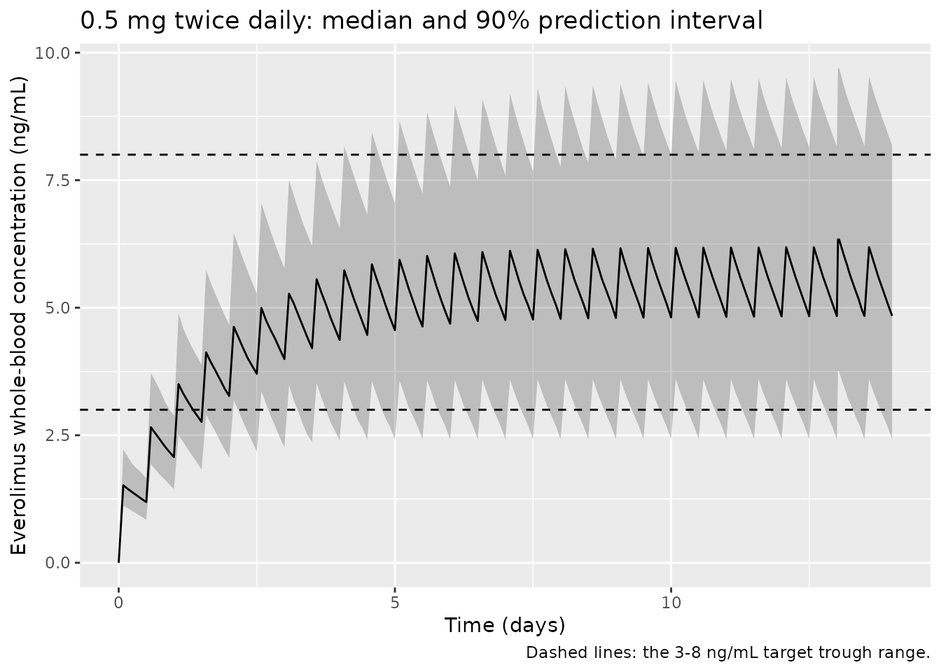
The cohort resembles the adult Table 1 population, every patient on the 0.5 mg twice-daily regimen the authors recommend (total daily dose 1.0 mg/day).
set.seed(2022)
n_sub <- 200
cohort <- tibble(
  id = seq_len(n_sub),
  WT = pmin(pmax(rlnorm(n_sub, log(57), 0.22), 34.5), 91),
  CRCL = pmin(pmax(rlnorm(n_sub, log(55.2), 0.5), 11.4), 223.7),
  SEXF = rbinom(n_sub, 1, 46 / 87),
  CONMED_FLUCONAZOLE = rbinom(n_sub, 1, 21 / 87),
  DOSE_EVEROLIMUS_MGD = 1.0
)
summary(cohort[, c("WT", "CRCL", "SEXF", "CONMED_FLUCONAZOLE")])
#>        WT             CRCL             SEXF      CONMED_FLUCONAZOLE
#>  Min.   :34.50   Min.   : 16.18   Min.   :0.00   Min.   :0.000
#>  1st Qu.:47.38   1st Qu.: 38.38   1st Qu.:0.00   1st Qu.:0.000
#>  Median :57.58   Median : 52.18   Median :1.00   Median :0.000
#>  Mean   :57.92   Mean   : 59.89   Mean   :0.54   Mean   :0.215
#>  3rd Qu.:67.15   3rd Qu.: 72.66   3rd Qu.:1.00   3rd Qu.:0.000
#>  Max.   :91.00   Max.   :212.27   Max.   :1.00   Max.   :1.000
Simulation: concentration-time profile over 14 days
mod <- readModelDb("Itohara_2022_everolimus")
rxode2::rxSetSeed(2022)

dose_times <- seq(0, 13.5 * 24, by = 12)
obs_times <- sort(unique(c(seq(0, 14 * 24, by = 2), 13 * 24 + seq(0, 12, by = 0.5))))
events <- bind_rows(
  tidyr::crossing(id = cohort$id, time = dose_times) |>
    mutate(evid = 1L, amt = 0.5, cmt = "depot"),
  tidyr::crossing(id = cohort$id, time = obs_times) |>
    mutate(evid = 0L, amt = 0, cmt = "central")
) |>
  left_join(cohort, by = "id") |>
  arrange(id, time, desc(evid)) |>
  select(id, time, evid, amt, cmt, everything())

sim <- rxode2::rxSolve(mod, events, returnType = "data.frame")
#> ℹ parameter labels from comments will be replaced by 'label()'
stopifnot(!anyNA(sim$Cc), n_distinct(sim$id) == n_sub)

sim |>
  group_by(time) |>
  summarise(
    p05 = quantile(Cc, 0.05), p50 = median(Cc), p95 = quantile(Cc, 0.95),
    .groups = "drop"
  ) |>
  ggplot(aes(time / 24, p50)) +
  geom_ribbon(aes(ymin = p05, ymax = p95), alpha = 0.25) +
  geom_line() +
  geom_hline(yintercept = c(3, 8), linetype = "dashed") +
  labs(
    x = "Time (days)", y = "Everolimus whole-blood concentration (ng/mL)",
    title = "0.5 mg twice daily: median and 90% prediction interval",
    caption = "Dashed lines: the 3-8 ng/mL target trough range."
  )
Replicate published figures
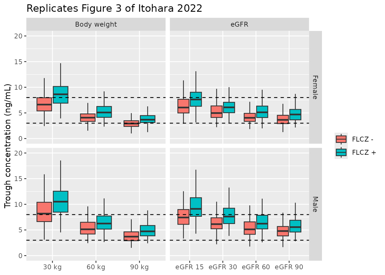
Figure 3: steady-state troughs by body weight, eGFR, sex and fluconazole
Figure 3 simulated troughs at 0.5 mg twice daily (5000 replicates per scenario; 200 here), varying body weight (30, 60, 90 kg) at eGFR 55.2, and eGFR (15, 30, 60, 90 mL/min/1.73 m^2) at 57 kg, for each sex with and without fluconazole.
scen <- bind_rows(
  tidyr::crossing(panel = "Body weight", WT = c(30, 60, 90), CRCL = 55.2),
  tidyr::crossing(panel = "eGFR", WT = 57, CRCL = c(15, 30, 60, 90))
) |>
  tidyr::crossing(SEXF = c(0L, 1L), CONMED_FLUCONAZOLE = c(0L, 1L)) |>
  mutate(scenario = row_number())

n_rep <- 200
fig3_events <- bind_rows(
  scen |> mutate(evid = 1L, time = 0, amt = 0.5, cmt = "depot", ii = 12, ss = 1L),
  scen |> mutate(evid = 0L, time = 12, amt = 0, cmt = "central", ii = 0, ss = 0L)
) |>
  tidyr::crossing(rep = seq_len(n_rep)) |>
  mutate(id = (scenario - 1L) * n_rep + rep, DOSE_EVEROLIMUS_MGD = 1.0) |>
  arrange(id, time, desc(evid)) |>
  select(id, time, evid, amt, cmt, ii, ss, everything())

rxode2::rxSetSeed(2023)
fig3 <- rxode2::rxSolve(
  mod, fig3_events,
  keep = c("panel", "scenario"), maxsteps = 500000L, returnType = "data.frame"
)
stopifnot(!anyNA(fig3$Cc), n_distinct(fig3$id) == nrow(scen) * n_rep)

fig3 <- fig3 |>
  mutate(
    sex = ifelse(SEXF == 1, "Female", "Male"),
    flcz = ifelse(CONMED_FLUCONAZOLE == 1, "FLCZ +", "FLCZ -"),
    level = ifelse(panel == "Body weight", paste(WT, "kg"), paste("eGFR", CRCL))
  )

ggplot(fig3, aes(factor(level, levels = unique(level)), Cc, fill = flcz)) +
  geom_boxplot(outlier.shape = NA) +
  geom_hline(yintercept = c(3, 8), linetype = "dashed") +
  facet_grid(sex ~ panel, scales = "free_x") +
  coord_cartesian(ylim = c(0, 20)) +
  labs(
    x = NULL, y = "Trough concentration (ng/mL)", fill = NULL,
    title = "Replicates Figure 3 of Itohara 2022"
  )
The typical-value troughs (no IIV, no residual error) behind the medians:
typ <- rxode2::rxSolve(
  rxode2::zeroRe(mod),
  fig3_events |> filter(rep == 1),
  keep = c("panel"), maxsteps = 500000L, returnType = "data.frame"
) |>
  filter(time == 12) |>
  transmute(
    panel, WT, eGFR = CRCL,
    sex = ifelse(SEXF == 1, "Female", "Male"),
    fluconazole = CONMED_FLUCONAZOLE, trough = signif(Cc, 3)
  )
#> ℹ parameter labels from comments will be replaced by 'label()'
#> ℹ omega/sigma items treated as zero: 'etalcl'
#> Warning: multi-subject simulation without without 'omega'
knitr::kable(typ)| panel | WT | eGFR | sex | fluconazole | trough |
|---|---|---|---|---|---|
| Body weight | 30 | 55.2 | Male | 0 | 8.38 |
| Body weight | 30 | 55.2 | Male | 1 | 10.50 |
| Body weight | 30 | 55.2 | Female | 0 | 6.57 |
| Body weight | 30 | 55.2 | Female | 1 | 8.26 |
| Body weight | 60 | 55.2 | Male | 0 | 5.11 |
| Body weight | 60 | 55.2 | Male | 1 | 6.36 |
| Body weight | 60 | 55.2 | Female | 0 | 4.03 |
| Body weight | 60 | 55.2 | Female | 1 | 5.04 |
| Body weight | 90 | 55.2 | Male | 0 | 3.82 |
| Body weight | 90 | 55.2 | Male | 1 | 4.74 |
| Body weight | 90 | 55.2 | Female | 0 | 3.02 |
| Body weight | 90 | 55.2 | Female | 1 | 3.77 |
| eGFR | 57 | 15.0 | Male | 0 | 7.71 |
| eGFR | 57 | 15.0 | Male | 1 | 9.52 |
| eGFR | 57 | 15.0 | Female | 0 | 6.13 |
| eGFR | 57 | 15.0 | Female | 1 | 7.61 |
| eGFR | 57 | 30.0 | Male | 0 | 6.33 |
| eGFR | 57 | 30.0 | Male | 1 | 7.84 |
| eGFR | 57 | 30.0 | Female | 0 | 5.01 |
| eGFR | 57 | 30.0 | Female | 1 | 6.24 |
| eGFR | 57 | 60.0 | Male | 0 | 5.17 |
| eGFR | 57 | 60.0 | Male | 1 | 6.44 |
| eGFR | 57 | 60.0 | Female | 0 | 4.07 |
| eGFR | 57 | 60.0 | Female | 1 | 5.10 |
| eGFR | 57 | 90.0 | Male | 0 | 4.59 |
| eGFR | 57 | 90.0 | Male | 1 | 5.73 |
| eGFR | 57 | 90.0 | Female | 0 | 3.60 |
| eGFR | 57 | 90.0 | Female | 1 | 4.52 |
The paper states that the median trough exceeded the 8 ng/mL upper target for light men and fell below the 3 ng/mL lower target for heavy women not taking fluconazole, with the rest almost within range (Results ‘Monte Carlo simulation’). The packaged model reproduces the direction of both extremes; the assertions below check them on the typical values, which are deterministic.
typ_val <- function(p, w, g, s, f) {
  typ$trough[typ$panel == p & typ$WT == w & typ$eGFR == g & typ$sex == s &
    typ$fluconazole == f]
}
light_male <- typ_val("Body weight", 30, 55.2, "Male", 0)
heavy_female <- typ_val("Body weight", 90, 55.2, "Female", 0)
c(light_male = light_male, heavy_female = heavy_female)
#>   light_male heavy_female
#>         8.38         3.02
stopifnot(
  light_male > 8,
  # The heavy-woman typical trough sits right on the 3 ng/mL boundary
  # (about 3.0 ng/mL), so the check is against a small band, not "< 3".
  heavy_female < 3.3,
  heavy_female < min(typ$trough[typ$sex == "Male"])
)
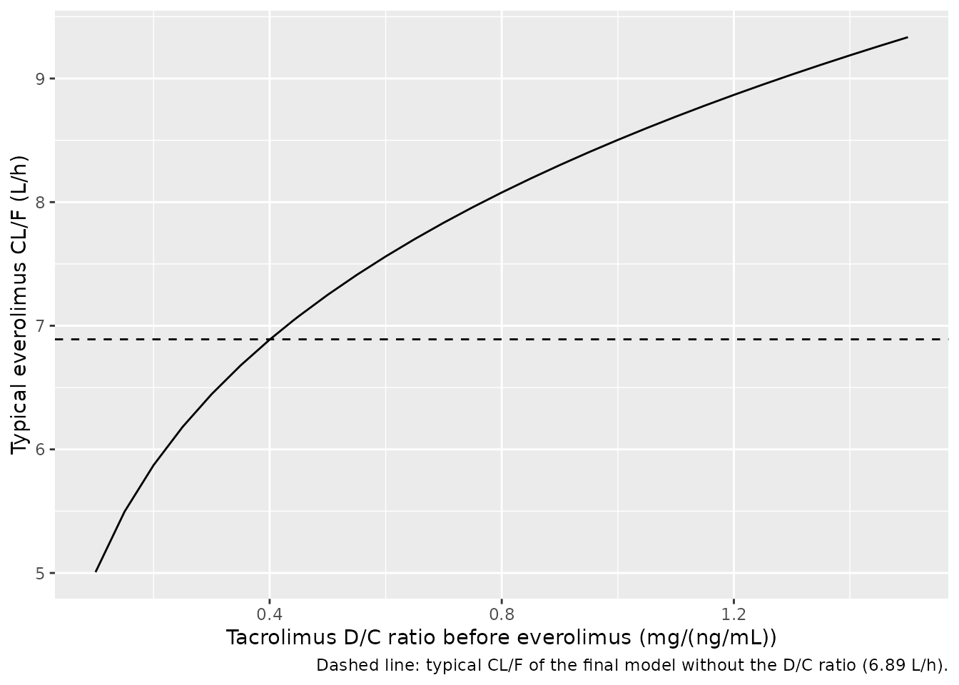
Prior tacrolimus D/C ratio and everolimus CL/F (Figure 4)
Figure 4 related the post-hoc everolimus CL/F to the tacrolimus D/C ratio (R^2 = 0.330). The prior-tacrolimus model turns that into a covariate: typical CL/F for a 57-kg man on 1 mg/day with eGFR 55.2 and no fluconazole:
mod_tac <- readModelDb("Itohara_2022_everolimus_prior_tacrolimus")
dc <- tibble(TAC_DOSE_TROUGH_RATIO_BL = sort(c(0.44, seq(0.1, 1.5, by = 0.05)))) |>
  mutate(
    id = row_number(), time = 0, evid = 0L, amt = 0, cmt = "central",
    WT = 57, DOSE_EVEROLIMUS_MGD = 1, CRCL = 55.2, SEXF = 0L, CONMED_FLUCONAZOLE = 0L
  ) |>
  select(id, time, evid, amt, cmt, everything())
dc_cl <- rxode2::rxSolve(rxode2::zeroRe(mod_tac), dc, returnType = "data.frame")
#> ℹ parameter labels from comments will be replaced by 'label()'
#> ℹ omega/sigma items treated as zero: 'etalcl'
#> Warning: multi-subject simulation without without 'omega'

ggplot(dc_cl, aes(TAC_DOSE_TROUGH_RATIO_BL, cl)) +
  geom_line() +
  geom_hline(yintercept = 6.89, linetype = "dashed") +
  labs(
    x = "Tacrolimus D/C ratio before everolimus (mg/(ng/mL))",
    y = "Typical everolimus CL/F (L/h)",
    caption = "Dashed line: typical CL/F of the final model without the D/C ratio (6.89 L/h)."
  )
PKNCA validation
Steady-state NCA over one 12-h dosing interval of 0.5 mg twice daily for the virtual cohort, grouped by sex and fluconazole use. The paper reports no NCA values, so the check is internal: PKNCA’s AUC over the interval must match dose / CL for each simulated subject.
treat <- cohort |>
  transmute(id, treatment = paste(ifelse(SEXF == 1, "Female", "Male"),
    ifelse(CONMED_FLUCONAZOLE == 1, "FLCZ +", "FLCZ -"),
    sep = ", "
  ))

ss_events <- bind_rows(
  tibble(id = cohort$id, time = 0, evid = 1L, amt = 0.5, cmt = "depot", ii = 12, ss = 1L),
  tidyr::crossing(id = cohort$id, time = seq(0, 12, by = 0.25)) |>
    mutate(evid = 0L, amt = 0, cmt = "central", ii = 0, ss = 0L)
) |>
  left_join(cohort, by = "id") |>
  arrange(id, time, desc(evid)) |>
  select(id, time, evid, amt, cmt, ii, ss, everything())

rxode2::rxSetSeed(2024)
sim_ss <- rxode2::rxSolve(mod, ss_events, maxsteps = 500000L, returnType = "data.frame")
stopifnot(!anyNA(sim_ss$Cc), n_distinct(sim_ss$id) == n_sub)

conc <- sim_ss |>
  filter(!is.na(Cc)) |>
  left_join(treat, by = "id") |>
  select(id, time, Cc, treatment)
dose <- tibble(id = cohort$id, time = 0, amt = 0.5) |>
  left_join(treat, by = "id")

o_conc <- PKNCA::PKNCAconc(conc, Cc ~ time | treatment + id)
o_dose <- PKNCA::PKNCAdose(dose, amt ~ time | treatment + id)
intervals <- data.frame(
  start = 0, end = 12,
  cmax = TRUE, cmin = TRUE, tmax = TRUE, auclast = TRUE
)
nca <- PKNCA::pk.nca(PKNCA::PKNCAdata(o_conc, o_dose, intervals = intervals))
summary(nca)
#>  start end      treatment  N     auclast        cmax        cmin
#>      0  12 Female, FLCZ - 85 60.2 [37.5] 5.81 [34.2] 4.23 [42.0]
#>      0  12 Female, FLCZ + 23 70.3 [43.3] 6.65 [39.4] 5.06 [48.4]
#>      0  12   Male, FLCZ - 72 73.2 [31.4] 6.85 [28.8] 5.34 [34.9]
#>      0  12   Male, FLCZ + 20  108 [45.4] 9.83 [42.5] 8.19 [48.8]
#>                  tmax
#>  0.750 [0.750, 0.750]
#>  0.750 [0.750, 0.750]
#>  0.750 [0.750, 0.750]
#>  0.750 [0.750, 0.750]
#>
#> Caption: auclast, cmax, cmin: geometric mean and geometric coefficient of variation; tmax: median and range; N: number of subjects
cl_by_id <- sim_ss |>
  group_by(id) |>
  summarise(cl = first(cl), .groups = "drop")
auc_chk <- as.data.frame(nca$result) |>
  filter(PPTESTCD == "auclast") |>
  mutate(id = as.integer(id)) |>
  left_join(cl_by_id, by = "id") |>
  # dose 0.5 mg / CL (L/h) = mg*h/L; x 1000 for ng*h/mL
  mutate(expected = 1000 * 0.5 / cl, pct_diff = 100 * (PPORRES / expected - 1))
summary(auc_chk$pct_diff)
#>     Min.  1st Qu.   Median     Mean  3rd Qu.     Max.
#> -0.16949 -0.09012 -0.07154 -0.07530 -0.05458 -0.02808
# Both sides use the same drawn parameters, so the only gap is the trapezoidal
# error of a 0.25-h grid over the ka = 6.07 /h absorption peak.
stopifnot(
  nrow(auc_chk) == n_sub,
  all(abs(auc_chk$pct_diff) < 3)
)
Assumptions and deviations
- Covariate distributions. The virtual cohort draws body weight and eGFR from log-normal distributions centred on the Table 1 medians and truncated to the Table 1 ranges; the paper reports only medians and ranges.
- IIV scale. Table 2 reports IIV as CV%; it is converted with omega^2 = log(CV^2 + 1) (0.271 -> 0.07085; 0.234 -> 0.05325).
-
Residual error. The combined error model is encoded
as
add(addSd) + prop(propSd)with the Table 2 values, the proportional term reported as a CV and the additive as an SD in ng/mL. -
Absorption.
kais the literature value the authors held constant; the data had no samples within 10 h of a dose, so neither the model nor this vignette constrains the absorption phase. -
Prior-tacrolimus model. The paper prints the CL/F
and Vd/F equations and the IIV and residual values, but no standard
errors.
kaand the allometric exponents are taken as held at the same values as in the final model. The tacrolimus D/C ratio is in mg/(ng/mL); the paper does not say whether its dose is the total daily dose, but the reported mean of 0.49 is consistent with a daily dose over a trough. The normalising value 0.44 is the one printed in the equation. - Paediatric extrapolation. The authors applied the adult model to 13 children (MPE -1.96 ng/mL overall, -0.706 without one infant outlier, Figure 5). No paediatric parameters were estimated, and the patient-level data needed to reproduce the MPE are not published, so it is not repeated here.
- Figure 3. The paper’s 5000 replicates per scenario are reduced to 200. The paper describes the heavy-woman, no-fluconazole median as below the 3 ng/mL target; the typical value from the packaged model sits at about 3.0 ng/mL, on the boundary.