Indisulam (Keizer 2015)
Source:vignettes/articles/Keizer_2015_indisulam.Rmd
Keizer_2015_indisulam.RmdModel and source
- Citation: Keizer RJ, Jansen RS, Rosing H, Thijssen B, Beijnen JH, Schellens JHM, Huitema ADR. Incorporation of concentration data below the limit of quantification in population pharmacokinetic analyses. Pharmacol Res Perspect. 2015;3(2):e00131. doi:10.1002/prp2.131.
- Description: Two-compartment linear IV population PK model for indisulam (E7070) in 34 adult solid-tumour patients receiving 250-525 mg/m2 as a 2-hour infusion in combination with irinotecan (Keizer 2015, Table 3, ‘All data’ column). This is the real-data model from a methodological study comparing four ways of handling concentrations below the limit of quantification; the ‘All data’ column is the paper’s advocated method, in which extrapolated concentrations between the limit of detection and the LLOQ are used as continuous observations. Interindividual variability is on clearance only; no covariates were investigated. Indisulam is known to have nonlinear (saturable) disposition, but nonlinearity was not supported by this limited data set and the fitted model is linear.
- Article: https://doi.org/10.1002/prp2.131 (open access, PMC4448983)
What this paper is, and which table was extracted
Keizer 2015 is primarily a methodological paper: it compares four ways of handling concentrations below the lower limit of quantification (LLOQ) in population PK analyses. It contains two parameter tables, and only one of them is a fitted model.
- Table 1 is NOT extracted. It lists the structural models and round parameter values (CL 5 L/h, V 50 L, Q2 10 L/h, V2 100 L, ka 0.5 /h) used to generate synthetic data sets for the simulation-and-reestimation study. These are simulation inputs that describe no drug, so they are not a pharmacometric model of anything and are deliberately not packaged.
- Table 3 IS extracted, and is what this vignette validates. The paper’s final section (“Real PopPK data set”) fits an original two-compartment linear population PK model to real clinical trial data for the anticancer agent indisulam (development code E7070), from a phase I dose-escalation study of indisulam combined with irinotecan (Ryan et al. 2005). Table 3 reports the complete final parameter set (structural, interindividual, residual) under each of the four BLQ-handling methods, and Figure 7 shows the corresponding bootstrap distributions.
The packaged model takes the “All data” column of Table 3. That is the method the paper advocates (extrapolated concentrations between the limit of detection and the LLOQ are used as ordinary continuous observations) and the one with by far the best estimation stability in this data set: 91.5% successful minimization and 85.7% successful covariance step, against 66.7% / 11.4% for the likelihood-based “LIKE” (Beal M3) method. The other three columns are reproduced below as a sensitivity comparison.
A separate, more elaborate semiphysiological model of indisulam’s nonlinear disposition exists (Zandvliet et al. 2006). It is not the model encoded here; Keizer 2015 states that nonlinearity was not supported by this limited data set.
Population
PK data came from 34 adult patients with advanced solid tumours receiving indisulam 250-525 mg/m^2 as a 2-hour intravenous infusion, in a phase I dose-escalation trial of indisulam plus irinotecan (Ryan et al. 2005). One PK curve per patient was available, sampled over 120 h. Excluding pre-first-dose samples, 231 PK samples were available, of which 17 (7.4%) were below the LLOQ. Plasma indisulam was assayed by a validated LC-MS/MS method over 0.1-20 microg/mL (Beumer et al. 2004); the limit of detection was taken as 30% of the LLOQ, i.e. 0.03 microg/mL.
Keizer 2015 reports no demographic table for this cohort (age, sex, weight and race are in the primary trial report, Ryan et al. 2005) and explicitly did not investigate covariates: “we only performed basic compartmental PK modeling on this limited data set, and, for example, the influence of covariates was not investigated.” The packaged model therefore carries no covariates.
The same information is available programmatically via the model’s
population metadata
(readModelDb("Keizer_2015_indisulam")()$population).
Source trace
Every value below is the “All data” column of Table 3 (page 9 of the
article). The per-parameter origin is also recorded as an in-file
comment next to each ini() entry in
inst/modeldb/specificDrugs/Keizer_2015_indisulam.R.
| Equation / parameter | Value | Source location |
|---|---|---|
lcl |
log(0.828) |
Table 3, row CL (L/h), “All data” column |
lvc |
log(5.63) |
Table 3, row V (L), “All data” column |
lq |
log(1.88) |
Table 3, row Q (L/h), “All data” column |
lvp |
log(12.6) |
Table 3, row Vper (L), “All data” column |
etalcl |
0.367236 |
Table 3, row eta_CL, “All data” column = 60.6%;
0.606^2
|
propSd |
0.267 |
Table 3, row sigma_prop, “All data” column = 26.7% |
addSd |
0.0364 |
Table 3, row sigma_add (mg/L), “All data” column |
| Two-compartment linear IV structure | n/a | “Real data sets”: “a two-compartment linear model showed a better fit than a linear one-compartment model” |
| IIV on CL only | n/a | Table 3 reports eta_CL and no other random effect |
| Combined additive + proportional residual | n/a | Table 3 reports both sigma_add and
sigma_prop; Methods: “A combined proportional and additive
error model was used” |
| No covariates | n/a | Methods, “Real PopPK data set”: covariates “not investigated” |
Note on the interindividual-variability scale
Table 3 labels the random-effect row eta_CL and reports
it as a percentage (60.6%), in exactly the same percentage style as the
sigma_prop row directly beneath it (26.7%).
sigma_prop is unambiguously the proportional residual
standard deviation itself, so by parallel construction
eta_CL is read as the standard deviation of the log-scale
random effect: omega = 0.606, hence
etalcl ~ 0.606^2 = 0.367236. The paper’s own simulation
section uses the same convention, defining the simulated between-subject
variability as “25%” (i.e. omega = 0.25). Reading 60.6% instead as an
exact log-normal CV would give log(1 + 0.606^2) = 0.3127,
i.e. omega = 0.559, which is inconsistent with the
sigma_prop row.
Virtual cohort
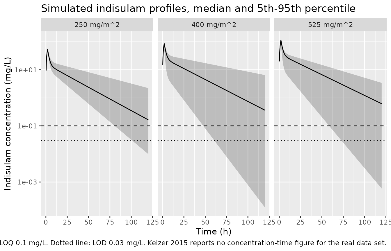
The original observed data are not publicly available. The cohort below spans the paper’s reported dose range (250, 400 and 525 mg/m^2), with 34 subjects per dose level to match the paper’s total N of 34 at each arm. Body surface area is not reported in Keizer 2015, so a standard adult 1.8 m^2 is assumed to convert mg/m^2 to the absolute mg doses the model consumes. The sampling grid covers the paper’s 120 h window; the real trial’s sampling times are not reported.
# `set.seed()` seeds R's RNG; `rxSetSeed()` seeds rxode2's, but only for a
# given solver-thread count. Every assertion below is therefore written either
# on a deterministic quantity (a solve against its own closed form) or with
# headroom that admits any cohort this model can produce.
set.seed(20150320)
rxode2::rxSetSeed(20150320)

BSA         <- 1.8    # m^2, assumed standard adult (not reported in the paper)
LLOQ        <- 0.1    # mg/L, assay LLOQ (Beumer 2004, cited by Keizer 2015)
LOD         <- 0.03   # mg/L, 30% of the LLOQ (Keizer 2015 Methods)
dose_levels <- c(250, 400, 525)   # mg/m^2, the paper's reported dose range

make_cohort <- function(n, dose_m2, id_offset = 0L) {
  obs <- c(
    seq(0, 4, by = 0.25), seq(4.5, 12, by = 0.5), seq(13, 24, by = 1),
    seq(28, 48, by = 4), seq(56, 120, by = 8)
  )
  rxode2::et(amt = dose_m2 * BSA, dur = 2, cmt = "central", id = seq_len(n)) |>
    rxode2::et(obs, cmt = "central") |>
    as.data.frame() |>
    dplyr::mutate(
      id         = id + id_offset,
      dose_group = sprintf("%d mg/m^2", dose_m2)
    )
}

events <- dplyr::bind_rows(
  make_cohort(34, dose_levels[1], id_offset =  0L),
  make_cohort(34, dose_levels[2], id_offset = 34L),
  make_cohort(34, dose_levels[3], id_offset = 68L)
)
stopifnot(!anyDuplicated(unique(events[, c("id", "time", "evid")])))
Simulation
mod <- readModelDb("Keizer_2015_indisulam")
sim <- rxode2::rxSolve(mod, events = events, keep = "dose_group")
Cc is the individual prediction (no residual error);
sim adds the combined additive plus proportional residual
error. With a 26.7% proportional residual term the simulated
observations go slightly negative in the far tail, so Cc is
used for the NCA and sim only where the residual error is
the point (the BLQ-fraction check).
sim |>
  dplyr::group_by(time, dose_group) |>
  dplyr::summarise(
    Q05 = quantile(Cc, 0.05), Q50 = median(Cc), Q95 = quantile(Cc, 0.95),
    .groups = "drop"
  ) |>
  dplyr::filter(time > 0) |>
  ggplot(aes(time, Q50)) +
  geom_ribbon(aes(ymin = Q05, ymax = Q95), alpha = 0.25) +
  geom_line() +
  geom_hline(yintercept = LLOQ, linetype = "dashed") +
  geom_hline(yintercept = LOD, linetype = "dotted") +
  facet_wrap(~dose_group) +
  scale_y_log10() +
  labs(
    x = "Time (h)", y = "Indisulam concentration (mg/L)",
    title = "Simulated indisulam profiles, median and 5th-95th percentile",
    caption = paste(
      "Dashed line: assay LLOQ 0.1 mg/L. Dotted line: LOD 0.03 mg/L.",
      "Keizer 2015 reports no concentration-time figure for the real data set."
    )
  )
Cross-check against Figure 7 (bootstrap distributions)
Keizer 2015 Figure 7 plots the bootstrap distributions of the four structural parameters, one panel per parameter, with all four BLQ methods overlaid. The panel axis ranges are printed on the figure and give an independent check that the Table 3 point estimates were transcribed correctly: every one of the 16 Table 3 structural values must fall inside its panel’s axis range.
tab3 <- tibble::tribble(
  ~method,    ~CL,   ~V,   ~Q,   ~Vper, ~etaCL, ~sigma_add, ~sigma_prop,
  "Discard",  0.823, 5.61, 1.90, 12.4,  0.623,  0.071,      0.258,
  "LLOQ/2",   0.819, 5.65, 1.89, 12.5,  0.615,  0.0344,     0.266,
  "LIKE",     0.822, 5.61, 1.90, 12.4,  0.618,  0.055,      0.261,
  "All data", 0.828, 5.63, 1.88, 12.6,  0.606,  0.0364,     0.267
)

# Axis ranges read off the four panels of Keizer 2015 Figure 7.
fig7_axes <- list(CL = c(0.4, 1.4), Q = c(1.2, 2.6), V = c(2, 9), Vper = c(8, 16))

inside <- vapply(names(fig7_axes), function(p) {
  rng <- fig7_axes[[p]]
  all(tab3[[p]] >= rng[1] & tab3[[p]] <= rng[2])
}, logical(1))

stopifnot(length(inside) == 4L, all(inside))
knitr::kable(
  tab3 |>
    dplyr::rename(
      "BLQ method"            = method,
      "CL (L/h)"              = CL,
      "V (L)"                 = V,
      "Q (L/h)"               = Q,
      "Vper (L)"              = Vper,
      "eta_CL"                = etaCL,
      "sigma_add (mg/L)"      = sigma_add,
      "sigma_prop"            = sigma_prop
    ),
  caption = paste(
    "Keizer 2015 Table 3, all four columns. The packaged model is the",
    "'All data' row. Every structural value lies inside its Figure 7 panel",
    "axis range."
  )
)| BLQ method | CL (L/h) | V (L) | Q (L/h) | Vper (L) | eta_CL | sigma_add (mg/L) | sigma_prop |
|---|---|---|---|---|---|---|---|
| Discard | 0.823 | 5.61 | 1.90 | 12.4 | 0.623 | 0.0710 | 0.258 |
| LLOQ/2 | 0.819 | 5.65 | 1.89 | 12.5 | 0.615 | 0.0344 | 0.266 |
| LIKE | 0.822 | 5.61 | 1.90 | 12.4 | 0.618 | 0.0550 | 0.261 |
| All data | 0.828 | 5.63 | 1.88 | 12.6 | 0.606 | 0.0364 | 0.267 |
PKNCA validation
For a linear model the NCA output has exact closed forms, so these are strict identity checks rather than tolerance comparisons: both sides use the same drawn parameters, and the only difference is trapezoidal and extrapolation error. Keizer 2015 reports no NCA parameters for the real data set, so there is no published NCA table to compare against.
sim_nca <- sim |>
  dplyr::filter(!is.na(Cc)) |>
  dplyr::select(id, time, Cc, dose_group)

# Guarantee a time = 0 anchor per subject (Cc = 0 pre-dose for an IV infusion).
sim_nca <- dplyr::bind_rows(
  sim_nca,
  sim_nca |> dplyr::distinct(id, dose_group) |> dplyr::mutate(time = 0, Cc = 0)
) |>
  dplyr::distinct(id, dose_group, time, .keep_all = TRUE) |>
  dplyr::arrange(id, dose_group, time)

dose_df <- events |>
  dplyr::filter(evid == 1) |>
  dplyr::select(id, time, amt, dose_group)

nca_res <- PKNCA::pk.nca(PKNCA::PKNCAdata(
  PKNCA::PKNCAconc(sim_nca, Cc ~ time | dose_group + id),
  PKNCA::PKNCAdose(dose_df, amt ~ time | dose_group + id),
  intervals = data.frame(
    start = 0, end = Inf,
    cmax = TRUE, tmax = TRUE, aucinf.obs = TRUE, half.life = TRUE
  )
))

nca_wide <- as.data.frame(nca_res) |>
  dplyr::select(id, dose_group, PPTESTCD, PPORRES) |>
  tidyr::pivot_wider(names_from = PPTESTCD, values_from = PPORRES)
stopifnot(nrow(nca_wide) == 102L, !anyNA(nca_wide$aucinf.obs))
Gate 1: AUC(0-inf) equals Dose / CL for every subject
Total exposure after a single IV dose of a linear model is exactly
Dose / CL, with no dependence on V, Q or Vper. This catches
a mis-transcribed clearance, a dose-unit error, or an infusion that
failed to deliver its full amount.
subj <- sim |> dplyr::distinct(id, cl, kel, k12, k21)

chk <- nca_wide |>
  dplyr::left_join(dose_df |> dplyr::distinct(id, amt), by = "id") |>
  dplyr::left_join(subj, by = "id") |>
  dplyr::mutate(
    auc_closed_form = amt / cl,
    auc_pct_diff    = 100 * (aucinf.obs - auc_closed_form) / auc_closed_form
  )

stopifnot(nrow(chk) == 102L, all(abs(chk$auc_pct_diff) < 0.5))
sprintf("AUCinf vs Dose/CL: max |%% difference| = %.4f%% over %d subjects",
        max(abs(chk$auc_pct_diff)), nrow(chk))
#> [1] "AUCinf vs Dose/CL: max |% difference| = 0.1154% over 102 subjects"
Gate 2: terminal half-life equals the closed-form beta half-life
Because interindividual variability sits on CL only, each subject has
a different terminal half-life. The check is therefore per
subject, against that subject’s own micro-constants:
beta = 0.5 * (k10 + k12 + k21 - sqrt((k10 + k12 + k21)^2 - 4 * k10 * k21)).
chk <- chk |>
  dplyr::mutate(
    ksum        = kel + k12 + k21,
    beta        = 0.5 * (ksum - sqrt(ksum^2 - 4 * kel * k21)),
    thalf_cf    = log(2) / beta,
    hl_pct_diff = 100 * (half.life - thalf_cf) / thalf_cf
  )

stopifnot(all(abs(chk$hl_pct_diff) < 2))
sprintf(paste("Terminal t1/2 vs closed form: max |%% difference| = %.4f%%;",
              "per-subject t1/2 spans %.1f to %.1f h"),
        max(abs(chk$hl_pct_diff)), min(chk$thalf_cf), max(chk$thalf_cf))
#> [1] "Terminal t1/2 vs closed form: max |% difference| = 0.4530%; per-subject t1/2 spans 6.9 to 75.9 h"
The typical-subject terminal half-life is 18.7 h. The wide per-subject spread is a direct consequence of the large reported interindividual variability on clearance (omega = 0.606).
Summary of simulated NCA by dose group
nca_wide |>
  dplyr::group_by(dose_group) |>
  dplyr::summarise(
    n           = dplyr::n(),
    cmax_med    = median(cmax),
    tmax_med    = median(tmax),
    aucinf_med  = median(aucinf.obs),
    thalf_med   = median(half.life),
    .groups = "drop"
  ) |>
  dplyr::rename(
    "Dose group"            = dose_group,
    "N"                     = n,
    "Cmax (mg/L)"           = cmax_med,
    "Tmax (h)"              = tmax_med,
    "AUC0-inf (mg*h/L)"     = aucinf_med,
    "t1/2 (h)"              = thalf_med
  ) |>
  knitr::kable(
    digits  = c(0, 0, 1, 2, 0, 1),
    caption = paste(
      "Median simulated NCA parameters by dose group. Keizer 2015 reports no",
      "NCA values for the real data set, so there is no published reference",
      "column."
    )
)| Dose group | N | Cmax (mg/L) | Tmax (h) | AUC0-inf (mg*h/L) | t1/2 (h) |
|---|---|---|---|---|---|
| 250 mg/m^2 | 34 | 52.5 | 2 | 514 | 17.9 |
| 400 mg/m^2 | 34 | 85.0 | 2 | 900 | 19.2 |
| 525 mg/m^2 | 34 | 112.4 | 2 | 1265 | 20.3 |
Reproducing the paper’s central real-data claim
Keizer 2015 concludes of the real indisulam data set (7.4% BLQ): “For all four BLOQ methods that were evaluated, the parameter estimates for this model were very similar”, and the Figure 7 bootstrap distributions “showed no sign of differences in mean parameter estimates or precision between the evaluated BLOQ methods.”
Running the packaged model with each of the four Table 3 parameter columns turns that qualitative claim into exposure numbers. The typical-value profiles are compared at 400 mg/m^2 (the middle of the reported dose range).
DOSE_MG <- 400 * BSA
ev_typ  <- rxode2::et(amt = DOSE_MG, dur = 2, cmt = "central") |>
  rxode2::et(seq(0, 240, by = 0.05), cmt = "central")

blq_cmp <- lapply(seq_len(nrow(tab3)), function(i) {
  r <- tab3[i, ]
  m <- mod |>
    rxode2::ini(
      lcl = log(r$CL), lvc = log(r$V), lq = log(r$Q), lvp = log(r$Vper)
    ) |>
    rxode2::zeroRe()
  s    <- rxode2::rxSolve(m, ev_typ, returnType = "data.frame")
  ksum <- r$CL / r$V + r$Q / r$V + r$Q / r$Vper
  beta <- 0.5 * (ksum - sqrt(ksum^2 - 4 * (r$CL / r$V) * (r$Q / r$Vper)))
  tibble::tibble(
    method = r$method,
    Cmax   = max(s$Cc),
    AUCinf = DOSE_MG / r$CL,
    thalf  = log(2) / beta,
    t_LLOQ = max(s$time[s$Cc >= LLOQ]),
    t_LOD  = max(s$time[s$Cc >= LOD])
  )
}) |> dplyr::bind_rows()

spread <- function(x) 100 * diff(range(x)) / mean(x)
stopifnot(
  nrow(blq_cmp) == 4L,
  # The paper's claim is that the four methods agree. At 7.4% BLQ censoring
  # they agree to ~1% on every exposure metric; 5% leaves ample headroom
  # while still going red if a column were mis-transcribed.
  spread(blq_cmp$Cmax)   < 5,
  spread(blq_cmp$AUCinf) < 5,
  spread(blq_cmp$thalf)  < 5
)

blq_cmp |>
  dplyr::rename(
    "BLQ method"            = method,
    "Cmax (mg/L)"           = Cmax,
    "AUC0-inf (mg*h/L)"     = AUCinf,
    "t1/2 (h)"              = thalf,
    "Time to LLOQ (h)"      = t_LLOQ,
    "Time to LOD (h)"       = t_LOD
  ) |>
  knitr::kable(
    digits  = c(0, 2, 1, 2, 1, 1),
    caption = paste(
      "Typical-value exposure at 400 mg/m^2 under each of the four Table 3",
      "parameter columns. Agreement to about 1% reproduces the paper's",
      "conclusion that at 7.4% BLQ censoring the handling method does not",
      "matter."
    )
)| BLQ method | Cmax (mg/L) | AUC0-inf (mg*h/L) | t1/2 (h) | Time to LLOQ (h) | Time to LOD (h) |
|---|---|---|---|---|---|
| Discard | 84.73 | 874.8 | 18.54 | 150.1 | 182.3 |
| LLOQ/2 | 84.49 | 879.1 | 18.78 | 151.8 | 184.4 |
| LIKE | 84.74 | 875.9 | 18.56 | 150.2 | 182.5 |
| All data | 84.64 | 869.6 | 18.74 | 151.1 | 183.7 |
What the “All data” method buys, in hours of observable curve
The paper’s premise is that concentrations between the LOD and the
LLOQ are real measurements that should not be discarded. With the
packaged model the value of that window is exactly computable: in the
terminal phase the concentration decays as exp(-beta * t),
so extending the usable range from the LLOQ down to the LOD (30% of the
LLOQ) adds log(LLOQ / LOD) / beta hours of observable
curve, independent of dose.
beta_typ <- {
  ksum <- 0.828 / 5.63 + 1.88 / 5.63 + 1.88 / 12.6
  0.5 * (ksum - sqrt(ksum^2 - 4 * (0.828 / 5.63) * (1.88 / 12.6)))
}
window_closed_form <- log(LLOQ / LOD) / beta_typ
window_simulated   <- blq_cmp$t_LOD[blq_cmp$method == "All data"] -
                      blq_cmp$t_LLOQ[blq_cmp$method == "All data"]

# Identity check: the simulated window extension must match the closed form
# to within the 0.05 h resolution of the observation grid.
stopifnot(abs(window_simulated - window_closed_form) < 0.1)
sprintf(paste("Extending observations from the LLOQ (%.2f mg/L) down to the",
              "LOD (%.2f mg/L) adds %.1f h of observable curve",
              "(closed form %.1f h)"),
        LLOQ, LOD, window_simulated, window_closed_form)
#> [1] "Extending observations from the LLOQ (0.10 mg/L) down to the LOD (0.03 mg/L) adds 32.6 h of observable curve (closed form 32.5 h)"
For a 120 h sampling window that is a substantial fraction of the study duration, which is why the method matters most when censoring is heavy. In this particular data set censoring was light (7.4%), and correspondingly the four methods agreed.
Corroborating the reported 7.4% BLQ fraction
This is an order-of-magnitude corroboration rather than a strict gate: the real trial’s sampling times are not reported, and the BLQ fraction depends strongly on how late and how densely samples were drawn. It is nevertheless sensitive to a concentration-unit error or a badly wrong clearance, either of which would move it by orders of magnitude.
blq_obs <- sim |>
  dplyr::mutate(obs = pmax(sim, 0)) |>
  dplyr::filter(time > 0) |>
  dplyr::summarise(
    n_samples = dplyr::n(),
    pct_blq   = 100 * mean(obs < LLOQ),
    pct_lod   = 100 * mean(obs < LOD)
  )

stopifnot(blq_obs$pct_blq > 0.2, blq_obs$pct_blq < 25)
sprintf(paste("Simulated: %.1f%% of samples below the LLOQ and %.1f%% below",
              "the LOD, against 17/231 = 7.4%% BLQ reported for the real",
              "data set"),
        blq_obs$pct_blq, blq_obs$pct_lod)
#> [1] "Simulated: 2.5% of samples below the LLOQ and 1.1% below the LOD, against 17/231 = 7.4% BLQ reported for the real data set"
Assumptions and deviations
- Only the “All data” column of Table 3 is packaged. The four columns are the same structural model refitted under four BLQ-handling methods. “All data” is the paper’s advocated method and had the best estimation stability (91.5% successful minimization, 85.7% successful covariance step). The other three columns are carried in this vignette as a sensitivity comparison, not as separate model files, because they are not distinct models.
- Table 1 is deliberately not extracted. Its values (CL 5 L/h, V 50 L, Q2 10 L/h, V2 100 L, ka 0.5 /h) are inputs used to generate synthetic data for the simulation study and correspond to no real drug.
-
Interindividual-variability scale.
eta_CL = 60.6%in Table 3 is read as the log-scale standard deviation (omega = 0.606, variance 0.367236) rather than as an exact log-normal CV (which would give omega = 0.559). The reasoning is in “Note on the interindividual-variability scale” above: the row sits in the same percentage style assigma_prop, which is unambiguously a standard deviation, and the paper’s simulation section uses the same convention. -
No interindividual variability on V, Q or Vper.
Table 3 reports only
eta_CL, so the other three structural parameters have no random effect. This is faithful to the source, not a simplification. - No covariates. The paper states explicitly that covariate effects were not investigated for this data set.
- Body surface area 1.8 m^2 is assumed to convert the paper’s mg/m^2 doses into the absolute mg the model consumes. Keizer 2015 reports no BSA distribution for this cohort. Nothing validated here depends on the choice: the closed-form gates are dose-normalised identities and the BLQ-method comparison is run at a single dose.
- The sampling grid is invented. The paper reports only that one PK curve per patient was obtained over 120 h. The grid used here is dense in the distribution phase and sparse in the terminal phase, which is why the simulated BLQ fraction (about 2.5%) sits below the reported 7.4%.
- Cohort size. 34 subjects per dose level at three dose levels (102 total). The paper’s 34 patients were distributed across the escalation levels rather than replicated at each.
- Demographics are not reproduced. Age, sex, weight and race for this cohort are in the primary trial report (Ryan et al. 2005), not in Keizer 2015, and no model parameter depends on them.
- Linear disposition. Indisulam is known to have saturable, nonlinear pharmacokinetics (Zandvliet et al. 2006), but nonlinearity and additional peripheral compartments were not supported by this data set, so the packaged model is linear as fitted. It should not be extrapolated far outside the 250-525 mg/m^2 range studied here.
- All parameter values come from the paper’s own Table 3. No value was taken from a figure, from correspondence, or from an upstream model.