Tramadol and O-desmethyltramadol in older patients (Al-Qurain 2022)
Source:vignettes/articles/AlQurain_2022_tramadol.Rmd
AlQurain_2022_tramadol.RmdModel and source
#> ℹ parameter labels from comments will be replaced by 'label()'- Citation: Al-Qurain AA, Upton RN, Tadros R, Roberts MS, Wiese MD. Population Pharmacokinetic Model for Tramadol and O-desmethyltramadol in Older Patients. Eur J Drug Metab Pharmacokinet. 2022;47(3):387-402. doi:10.1007/s13318-022-00756-x
- Description: Joint parent-and-metabolite population PK model for extended-release oral tramadol and its active CYP2D6-derived metabolite O-desmethyltramadol (ODT, M1) in older hospital inpatients (Al-Qurain 2022). Two-compartment tramadol disposition with first-order absorption and linear elimination; CL/F is the total apparent tramadol clearance, and ODT is formed at a first-order rate (Kt) from the tramadol central amount into a one-compartment apparent ODT pool that shares the tramadol central volume and is cleared linearly (CLm/F). Because the fraction of tramadol metabolised to ODT is not identifiable, the ODT pool is scaled by it and the formation term does not deplete tramadol. The Identification of Seniors At Risk (ISAR) frailty score raises the tramadol inter-compartmental clearance, and Cockcroft-Gault creatinine clearance raises both the tramadol apparent clearance and the peripheral volume, each through an uncentred exponential term.
- Article: https://doi.org/10.1007/s13318-022-00756-x
Al-Qurain et al. fitted tramadol and its active CYP2D6-formed metabolite O-desmethyltramadol (ODT) jointly in 21 older hospital inpatients taking extended-release oral tramadol, using Monolix 2020 (SAEM). The final estimates are in Table 3 of the paper. The open-access supplement holds the structural-model and covariate-screening tables (Tables S1-S7) but no model code and no covariate equation, so several encoding choices below rest on the reasoning laid out in Assumptions and deviations.
A search on 2026-10-02 (Europe PMC, and the Crossref record for the DOI) found no erratum or correction notice for this article.
Population
21 patients aged 69-93 years (mean 83.2, SD 7.5) were recruited at the Royal Adelaide Hospital (Australia) between June and November 2019 (Table 1). 43% were male; body weight was 33-112 kg (mean 68.3). All had normal liver function tests. Renal function was wide-ranging: Cockcroft-Gault creatinine clearance (CrCL) 16-351 mL/min (mean 65.1, SD 69.1). The Identification of Seniors At Risk (ISAR) frailty score was 1-5 (mean 3, SD 1.2), and 38% took a CYP3A4 inhibitor and 38% a CYP2D6 inhibitor. Doses were 25 mg (n = 3), 50 mg (n = 6), 75 mg (n = 1) or 100 mg (n = 11). Up to five finger-prick volumetric absorptive microsamples were taken per patient within 12 h of a dose (99 samples in total, all above the 10 ng/mL limit of quantitation).
The same information is available programmatically via
readModelDb("AlQurain_2022_tramadol")()$population.
Model structure
Figure 1 of the paper: oral tramadol is absorbed first-order
(ka) into a central compartment (V1/F) that
exchanges with a peripheral compartment (V2/F,
Q) and is cleared linearly by CL/F. ODT is
formed at the first-order rate Kt from the tramadol central
amount into a one-compartment pool that shares the tramadol central
volume and is cleared by CLm/F.
CL/F is the total apparent tramadol
clearance, and the formation term does not deplete tramadol. Methods
2.4.2 states that the fraction of tramadol metabolised to ODT
(Fm) is not identifiable from parent-only oral dosing, and
that only Vm/(F km) and CLm/(F km) can be
determined; the ODT pool is therefore an apparent amount scaled by
1/Fm. This reading reproduces the paper’s steady-state VPC
(Figure 6) and the CrCL dependence of Figure 11, both shown below; a
mass-balance reading in which Kt also drains tramadol
reaches only about half of the Figure 6 medians and leaves CrCL almost
without effect (see Assumptions
and deviations).
Covariates enter as uncentred exponentials:
-
Q = 42.6 * exp(0.255 * ISAR)L/h -
CL/F = 6.04 * exp(0.00498 * CrCL)L/h -
V2/F = 379 * exp(0.0119 * CrCL)L
# The model defines a cl / vc pair, which rxode2 could replace with an analytic
# linCmt() solution, discarding the metabolite compartment. Confirm the four ODE
# states are present.
stopifnot(identical(
  rxode2::rxState(rxode2::rxModelVars(ui)),
  c("depot", "central", "peripheral1", "central_m1")
))
Source trace
| Quantity | Value in model | Source |
|---|---|---|
ka |
2.96 1/h | Table 3, final model, ‘K a, /h’ |
V1/F (vc) |
373 L | Table 3, ‘V 1 / F , l’ = 0.373 (x 1000; see Assumptions) |
Q |
42.6 L/h at ISAR 0 | Table 3, ‘Q , l/h’ = 0.0426 (x 1000) |
| ISAR effect on Q | 0.255 | Table 3, ‘ISAR effect on Q’ |
V2/F (vp) |
379 L at CrCL 0 | Table 3, ‘V 2 / F , l’ = 0.379 (x 1000) |
| CrCL effect on V2/F | 0.0119 per mL/min | Table 3, ‘CrCL effect on V 2 / F’ |
CL/F (cl) |
6.04 L/h at CrCL 0 | Table 3, ‘CL/ F , l/h’ = 0.00604 (x 1000) |
| CrCL effect on CL/F | 0.00498 per mL/min | Table 3, ‘CrCL effect on CL/F’ |
Kt (kmet) |
0.0492 1/h | Table 3, ‘K t , l/h’ (rate constant per footnote) |
CLm/F (cl_m1) |
143 L/h | Table 3, ‘CL m / F , l/h’ = 0.143 (x 1000) |
| IIV (SD) ka, V1, Q, V2, CL, Kt, CLm | 0.378, 0.738, 0.0219, 0.974, 0.0661, 0.785, 0.216 | Table 3 ‘Omega’ rows; footnote: presented as SD |
| Tramadol proportional error | 0.157 | Table 3, ‘Tramadol, b (%)’ |
| ODT additive error | 5.19 ng/mL | Table 3, ‘O -desmethyltramadol, a (%)’ |
| ODT proportional error | 0.189 | Table 3, ‘O -desmethyltramadol, b (%)’ |
| Structure (2-cmt parent, 1-cmt metabolite, first-order absorption and formation) |
model() ODEs |
Figure 1; Methods 2.4.2; Results 3.3 |
| Formation does not deplete tramadol (Fm-scaled ODT pool) |
d/dt(central) has no kmet term |
Methods 2.4.2 identifiability statement; checked against Figures 6 and 11 |
| Log-normal IIV | exp(theta + eta) |
Methods 2.4.1, Eq. 1 |
| Covariate form | uncentred exp(beta * COV)
|
Not printed; Monolix default, checked against Figure 10 |
| Error models | proportional (tramadol), combined (ODT) | Results 3.3 |
Typical-value checks
The covariate model is algebraic, so the typical individual
parameters at any covariate value follow exactly from
ini():
mod_typ <- ui |> rxode2::zeroRe()
ini_vals <- ui$theta
typ <- data.frame(
  SCORE_ISAR = c(0, 3, 6, 3),
  CRCL = c(0, 65.1, 65.1, 120)
) |>
  dplyr::mutate(
    Q = exp(ini_vals[["lq"]] + ini_vals[["e_score_isar_q"]] * SCORE_ISAR),
    CL = exp(ini_vals[["lcl"]] + ini_vals[["e_crcl_cl"]] * CRCL),
    V2 = exp(ini_vals[["lvp"]] + ini_vals[["e_crcl_vp"]] * CRCL),
    t_half_terminal = log(2) * (exp(ini_vals[["lvc"]]) + V2) / CL
  )
typ |>
  dplyr::rename(
    "ISAR" = SCORE_ISAR,
    "CrCL (mL/min)" = CRCL,
    "Q (L/h)" = Q,
    "CL/F (L/h)" = CL,
    "V2/F (L)" = V2,
    "Approximate terminal t1/2 (h)" = t_half_terminal
  ) |>
knitr::kable(digits = 3)| ISAR | CrCL (mL/min) | Q (L/h) | CL/F (L/h) | V2/F (L) | Approximate terminal t1/2 (h) |
|---|---|---|---|---|---|
| 0 | 0.0 | 42.600 | 6.040 | 379.000 | 86.299 |
| 3 | 65.1 | 91.547 | 8.353 | 822.399 | 99.198 |
| 6 | 65.1 | 196.734 | 8.353 | 822.399 | 99.198 |
| 3 | 120.0 | 91.547 | 10.979 | 1580.563 | 123.334 |
# The covariate terms reproduce the cohort-mean values quoted in the
# covariateData notes (CL/F 8.3 L/h and V2/F 820 L at CrCL 65.1 mL/min).
stopifnot(
  abs(typ$CL[2] - 8.35) < 0.05,
  abs(typ$V2[2] / 822 - 1) < 0.01
)
The approximate terminal half-life, ln 2 (V1 + V2) / CL,
is long (several days) because CL/F is small relative to
the combined volume. Steady state is therefore reached only after weeks
of dosing, which the simulations below allow for.
At steady state ODT follows tramadol with its short own half-life, so
the typical ODT/tramadol concentration ratio is
Kt x V1 / CLm (the two species share the same volume):
Replicate Figure 10 (typical profiles by ISAR)
Figure 10 shows typical single-dose tramadol profiles at ISAR 0, 3 and 6 after 50 and 100 mg, with the dose given at 1 h on the figure axis. The CrCL used is not stated; the cohort mean 65.1 mL/min is used here (the single-dose peak is insensitive to CrCL, see Figure 11 below).
fig10_subj <- tidyr::crossing(
  SCORE_ISAR = c(0, 3, 6),
  dose_mg = c(50, 100)
) |>
  dplyr::mutate(id = dplyr::row_number(), CRCL = 65.1)

fig10_ev <- dplyr::bind_rows(
  fig10_subj |>
    dplyr::mutate(time = 1, amt = dose_mg, evid = 1L, cmt = "depot", dvid = NA_integer_),
  tidyr::crossing(fig10_subj, time = seq(0, 12, by = 0.05)) |>
    dplyr::mutate(amt = NA_real_, evid = 0L, cmt = "central", dvid = 1L)
) |>
  dplyr::arrange(id, time, dplyr::desc(evid))

fig10_sim <- rxode2::rxSolve(
  mod_typ,
  events = fig10_ev,
  keep = c("SCORE_ISAR", "dose_mg"),
  useLinCmt = FALSE
) |>
  as.data.frame()
#> ℹ omega/sigma items treated as zero: 'etalka', 'etalvc', 'etalq', 'etalvp', 'etalcl', 'etalkmet', 'etalcl_m1'
#> Warning: multi-subject simulation without without 'omega'

ggplot(fig10_sim, aes(time, Cc, colour = factor(dose_mg))) +
  geom_line() +
  facet_wrap(~ paste("ISAR =", SCORE_ISAR)) +
  scale_colour_manual(values = c("50" = "black", "100" = "red")) +
  labs(
    x = "Time (h)", y = "Tramadol concentration (ng/mL)", colour = "Dose (mg)",
    caption = "Replicates Figure 10 of Al-Qurain 2022."
  )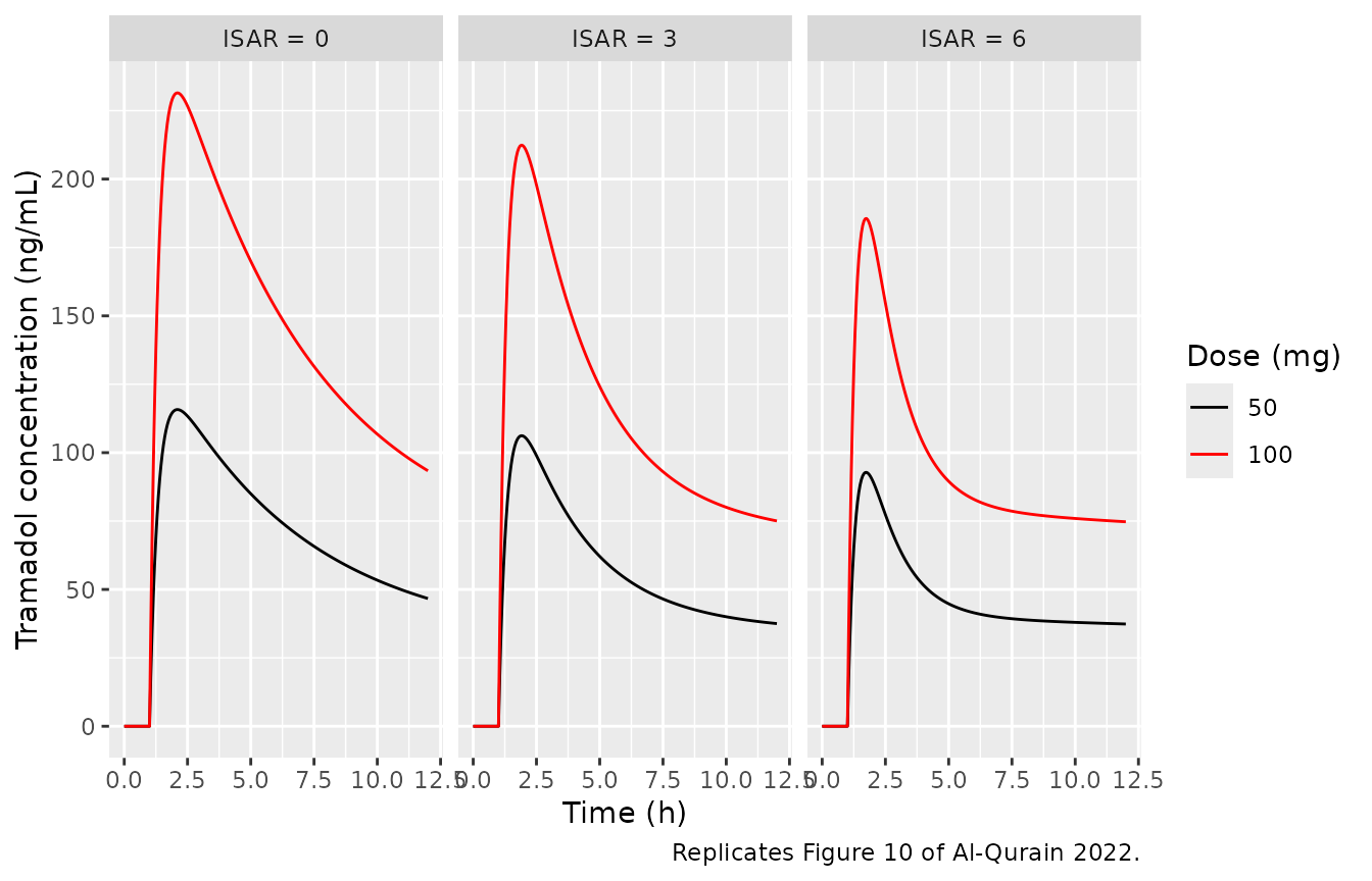
Peak concentrations after 100 mg, against values read off Figure 10 by the maintainers:
fig10_cmax <- fig10_sim |>
  dplyr::filter(dose_mg == 100) |>
  dplyr::group_by(SCORE_ISAR) |>
  dplyr::summarise(
    Cmax = max(Cc),
    C12 = Cc[abs(time - 12) < 1e-6],
    .groups = "drop"
  ) |>
  dplyr::mutate(
    Cmax_fig10 = c(240, 220, 195),
    C12_fig10 = c(90, 112, 115),
    pct_diff = 100 * (Cmax / Cmax_fig10 - 1),
    rel_to_isar0 = Cmax / Cmax[1],
    rel_to_isar0_fig10 = Cmax_fig10 / Cmax_fig10[1]
  )
fig10_cmax |>
  dplyr::select(
    SCORE_ISAR, Cmax, Cmax_fig10, pct_diff, rel_to_isar0, rel_to_isar0_fig10,
    C12, C12_fig10
  ) |>
  dplyr::rename(
    "ISAR" = SCORE_ISAR,
    "Simulated Cmax (ng/mL)" = Cmax,
    "Figure 10 Cmax (ng/mL)" = Cmax_fig10,
    "Cmax difference (%)" = pct_diff,
    "Simulated Cmax, relative to ISAR 0" = rel_to_isar0,
    "Figure 10 Cmax, relative to ISAR 0" = rel_to_isar0_fig10,
    "Simulated C at 12 h (ng/mL)" = C12,
    "Figure 10 C at 12 h (ng/mL)" = C12_fig10
  ) |>
knitr::kable(digits = 2)| ISAR | Simulated Cmax (ng/mL) | Figure 10 Cmax (ng/mL) | Cmax difference (%) | Simulated Cmax, relative to ISAR 0 | Figure 10 Cmax, relative to ISAR 0 | Simulated C at 12 h (ng/mL) | Figure 10 C at 12 h (ng/mL) |
|---|---|---|---|---|---|---|---|
| 0 | 231.51 | 240 | -3.54 | 1.00 | 1.00 | 93.37 | 90 |
| 3 | 212.39 | 220 | -3.46 | 0.92 | 0.92 | 75.05 | 112 |
| 6 | 185.59 | 195 | -4.83 | 0.80 | 0.81 | 74.74 | 115 |
# Deterministic typical-value solve against digitised figure values: the
# absolute peak within the reading error of the figure, and the ISAR-driven
# reduction in the peak (the covariate effect itself) within a few percent.
stopifnot(
  all(abs(fig10_cmax$pct_diff) < 10),
  all(abs(fig10_cmax$rel_to_isar0 - fig10_cmax$rel_to_isar0_fig10) < 0.03)
)
The peak and its ISAR dependence are reproduced: the peaks are within
5% of the figure and the ratio to ISAR 0 matches to two decimals, which
supports the uncentred covariate form (centring ISAR on 3 would lower Q
at ISAR 0 by a factor of exp(-0.765) = 0.47 and move the
ISAR 0 peak the other way). The 12 h concentration matches at ISAR 0,
but the figure keeps rising with ISAR at 12 h while the simulation does
not. The figure does not state the CrCL it used, and the late tail
depends strongly on CrCL through V2/F and
CL/F.
Figure 11 (CrCL)
Figure 11 shows a 50 or 100 mg dose given at 1 h on top of an existing concentration (about 400, 290 and 200 ng/mL before the 100 mg dose at CrCL 30, 75 and 120 mL/min). The prior regimen that produced those baselines, and the ISAR used, are not stated. Two things can be checked. First, the rise above baseline is about 220 ng/mL in all three panels, i.e. the single-dose peak does not depend on CrCL:
fig11_subj <- data.frame(id = 1:3, CRCL = c(30, 75, 120), SCORE_ISAR = 3, dose_mg = 100)
fig11_ev <- dplyr::bind_rows(
  fig11_subj |>
    dplyr::mutate(time = 0, amt = dose_mg, evid = 1L, cmt = "depot", dvid = NA_integer_),
  tidyr::crossing(fig11_subj, time = seq(0, 12, by = 0.05)) |>
    dplyr::mutate(amt = NA_real_, evid = 0L, cmt = "central", dvid = 1L)
) |>
  dplyr::arrange(id, time, dplyr::desc(evid))
fig11_sim <- rxode2::rxSolve(mod_typ, events = fig11_ev, keep = "CRCL", useLinCmt = FALSE) |>
  as.data.frame()
#> ℹ omega/sigma items treated as zero: 'etalka', 'etalvc', 'etalq', 'etalvp', 'etalcl', 'etalkmet', 'etalcl_m1'
#> Warning: multi-subject simulation without without 'omega'
fig11_cmax <- fig11_sim |>
  dplyr::group_by(CRCL) |>
  dplyr::summarise(Cmax = max(Cc), .groups = "drop")
knitr::kable(
  fig11_cmax |> dplyr::rename("CrCL (mL/min)" = CRCL, "Single-dose Cmax (ng/mL)" = Cmax),
  digits = 1
)| CrCL (mL/min) | Single-dose Cmax (ng/mL) |
|---|---|
| 30 | 213.5 |
| 75 | 212.1 |
| 120 | 210.9 |
Second, the pre-dose baselines fall about two-fold from CrCL 30 to 120 mL/min. Typical steady-state troughs after 100 mg every 12 or 24 hours (eight weeks of dosing, which is several terminal half-lives):
make_ss_events <- function(subj, tau, t_end, obs_tad) {
  n_dose <- floor(t_end / tau) + 1
  t_last <- tau * (n_dose - 1)
  dplyr::bind_rows(
    subj |>
      dplyr::mutate(
        time = 0, amt = dose_mg, evid = 1L, cmt = "depot",
        ii = tau, addl = n_dose - 1, dvid = NA_integer_
      ),
    tidyr::crossing(subj, time = t_last + obs_tad) |>
      dplyr::mutate(amt = NA_real_, evid = 0L, cmt = "central", ii = 0, addl = 0, dvid = 1L)
  ) |>
    dplyr::arrange(id, time, dplyr::desc(evid)) |>
    dplyr::mutate(t_last = t_last)
}
t_end <- 24 * 7 * 8
fig11_ss <- dplyr::bind_rows(lapply(c(12, 24), function(tau) {
  ev <- make_ss_events(fig11_subj, tau, t_end, 0)
  rxode2::rxSolve(mod_typ, events = ev, keep = "CRCL", useLinCmt = FALSE, maxsteps = 500000L) |>
    as.data.frame() |>
    dplyr::mutate(interval = paste0("every ", tau, " h"))
})) |>
  dplyr::select(interval, CRCL, trough = Cc) |>
  dplyr::mutate(baseline_fig11 = rep(c(400, 290, 200), 2))
#> ℹ omega/sigma items treated as zero: 'etalka', 'etalvc', 'etalq', 'etalvp', 'etalcl', 'etalkmet', 'etalcl_m1'
#> Warning: multi-subject simulation without without 'omega'
#> ℹ omega/sigma items treated as zero: 'etalka', 'etalvc', 'etalq', 'etalvp', 'etalcl', 'etalkmet', 'etalcl_m1'
#> Warning: multi-subject simulation without without 'omega'
fig11_ss |>
  dplyr::rename(
    "Dosing interval" = interval,
    "CrCL (mL/min)" = CRCL,
    "Simulated steady-state trough (ng/mL)" = trough,
    "Figure 11 baseline (ng/mL)" = baseline_fig11
  ) |>
knitr::kable(digits = 0)| Dosing interval | CrCL (mL/min) | Simulated steady-state trough (ng/mL) | Figure 11 baseline (ng/mL) |
|---|---|---|---|
| every 12 h | 30 | 1109 | 400 |
| every 12 h | 75 | 874 | 290 |
| every 12 h | 120 | 686 | 200 |
| every 24 h | 30 | 529 | 400 |
| every 24 h | 75 | 419 | 290 |
| every 24 h | 120 | 330 | 200 |
span <- fig11_ss |>
  dplyr::group_by(interval) |>
  dplyr::summarise(span = trough[CRCL == 30] / trough[CRCL == 120], .groups = "drop")
span
#> # A tibble: 2 × 2
#>   interval    span
#>   <chr>      <dbl>
#> 1 every 12 h  1.62
#> 2 every 24 h  1.60

# CrCL acts on CL/F, which is the only tramadol clearance, so the trough must
# fall materially between CrCL 30 and 120 mL/min (Figure 11: about 2-fold). A
# structure in which ODT formation also drains tramadol gives only about 1.2-fold
# here, because CL/F is then a minor share of the total clearance.
stopifnot(all(span$span > 1.4))
The baselines span about 1.6-fold across CrCL 30-120 mL/min in the simulation against about 2-fold in Figure 11. The absolute baselines depend on the unstated regimen, so they are not asserted.
Virtual cohort
Covariates are drawn to resemble Table 1. ISAR is an integer 1-5 with probabilities 0.1, 0.2, 0.4, 0.2, 0.1 (mean 3, SD 1.1). CrCL is log-normal with median 48 mL/min and log-SD 0.75, truncated to the observed 16-351 mL/min range (the reported mean 65 and SD 69 indicate a strong right skew). Doses follow the study mix (25, 50, 75, 100 mg in proportion 3 : 6 : 1 : 11).
n_vpc <- 200
draw_crcl <- function(n) {
  x <- stats::rlnorm(n * 3, log(48), 0.75)
  x <- x[x >= 16 & x <= 351]
  x[seq_len(n)]
}
vpc_subj <- data.frame(
  id = seq_len(n_vpc),
  SCORE_ISAR = sample(1:5, n_vpc, replace = TRUE, prob = c(0.1, 0.2, 0.4, 0.2, 0.1)),
  CRCL = draw_crcl(n_vpc),
  dose_mg = sample(c(25, 50, 75, 100), n_vpc, replace = TRUE, prob = c(3, 6, 1, 11) / 21)
)
summary(vpc_subj[, c("SCORE_ISAR", "CRCL", "dose_mg")])
#>    SCORE_ISAR        CRCL           dose_mg
#>  Min.   :1.00   Min.   : 16.15   Min.   : 25.00
#>  1st Qu.:2.00   1st Qu.: 32.75   1st Qu.: 50.00
#>  Median :3.00   Median : 52.78   Median : 75.00
#>  Mean   :2.97   Mean   : 71.32   Mean   : 71.25
#>  3rd Qu.:4.00   3rd Qu.: 88.45   3rd Qu.:100.00
#>  Max.   :5.00   Max.   :349.99   Max.   :100.00
Simulation: steady-state VPC (replicates Figure 6)
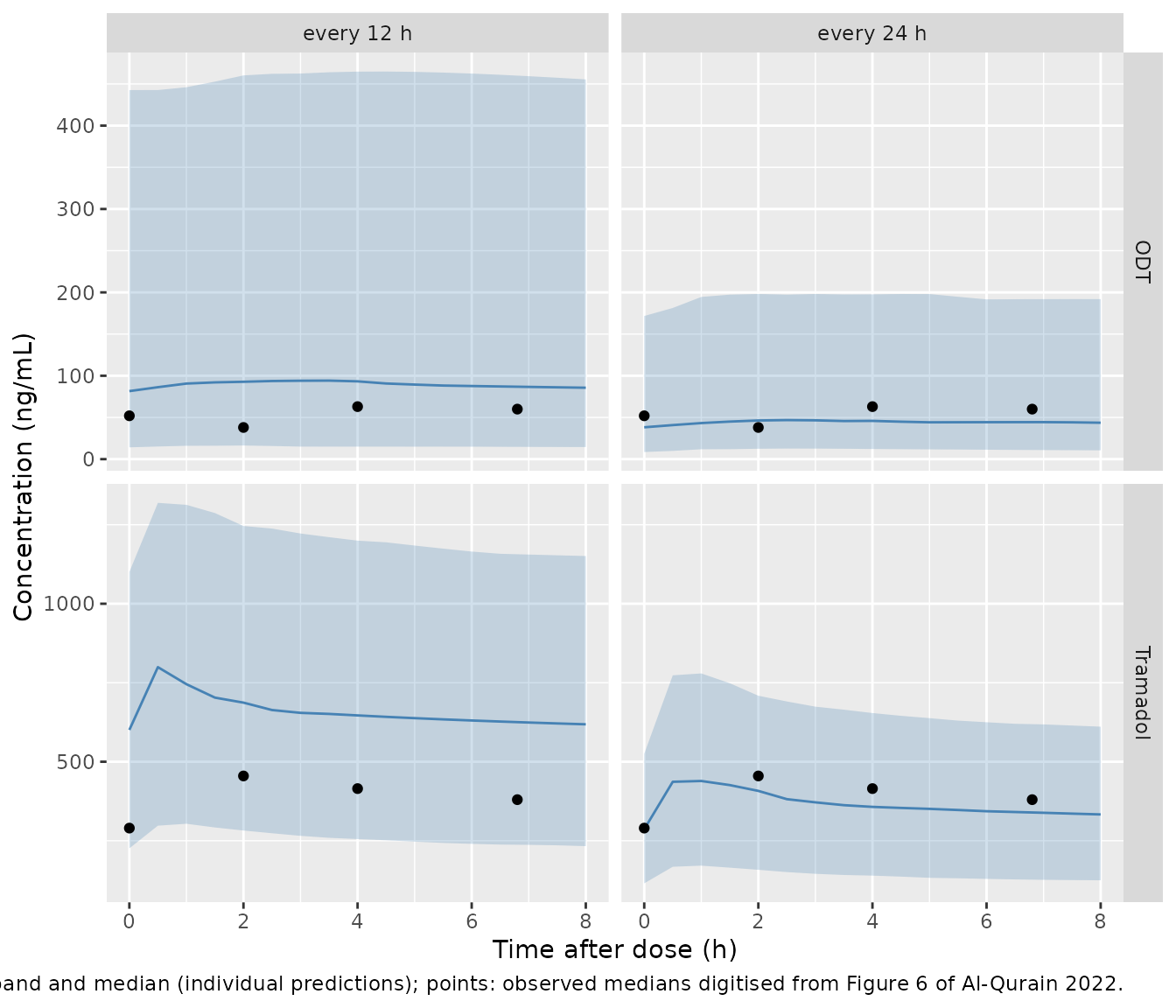
The paper’s VPC (Figure 6) plots concentrations 0-8 h after a dose in patients on established therapy. The long-term dosing interval is not reported, so the same cohort is simulated under both 12-hourly and once-daily dosing for eight weeks, and the last dosing interval is observed.
vpc_sim <- dplyr::bind_rows(lapply(c(12, 24), function(tau) {
  ev <- make_ss_events(vpc_subj, tau, t_end, seq(0, 8, by = 0.5))
  rxode2::rxSolve(
    ui,
    events = ev,
    keep = c("SCORE_ISAR", "CRCL", "dose_mg", "t_last"),
    useLinCmt = FALSE,
    maxsteps = 500000L
  ) |>
    as.data.frame() |>
    dplyr::mutate(interval = paste0("every ", tau, " h"), tad = time - t_last)
}))
stopifnot(!anyNA(vpc_sim$Cc), !anyNA(vpc_sim$Cc_m1))
The bands below use individual predictions (Cc,
Cc_m1, between-subject variability without residual error).
Observed medians read off Figure 6 by the maintainers are overlaid as
points.
vpc_q <- vpc_sim |>
  dplyr::select(interval, id, tad, Tramadol = Cc, ODT = Cc_m1) |>
  tidyr::pivot_longer(c(Tramadol, ODT), names_to = "analyte", values_to = "conc") |>
  dplyr::group_by(interval, analyte, tad) |>
  dplyr::summarise(
    p10 = stats::quantile(conc, 0.1),
    p50 = stats::quantile(conc, 0.5),
    p90 = stats::quantile(conc, 0.9),
    .groups = "drop"
  )
fig6_obs <- data.frame(
  analyte = rep(c("Tramadol", "ODT"), each = 4),
  tad = rep(c(0, 2, 4, 6.8), 2),
  median_obs = c(290, 455, 415, 380, 52, 38, 63, 60)
)
ggplot(vpc_q, aes(tad)) +
  geom_ribbon(aes(ymin = p10, ymax = p90), fill = "steelblue", alpha = 0.25) +
  geom_line(aes(y = p50), colour = "steelblue") +
  geom_point(data = fig6_obs, aes(y = median_obs), colour = "black") +
  facet_grid(analyte ~ interval, scales = "free_y") +
  labs(
    x = "Time after dose (h)", y = "Concentration (ng/mL)",
    caption = paste(
      "Simulated 10th-90th percentile band and median (individual predictions);",
      "points: observed medians digitised from Figure 6 of Al-Qurain 2022."
    )
  )
vpc_cmp <- vpc_q |>
  dplyr::inner_join(
    fig6_obs |> dplyr::mutate(tad = round(tad * 2) / 2),
    by = c("analyte", "tad")
  ) |>
  dplyr::mutate(ratio_sim_obs = p50 / median_obs)
vpc_cmp |>
  dplyr::select(interval, analyte, tad, p50, median_obs, ratio_sim_obs) |>
  dplyr::arrange(analyte, interval, tad) |>
  dplyr::rename(
    "Dosing interval" = interval,
    "Analyte" = analyte,
    "Time after dose (h)" = tad,
    "Simulated median (ng/mL)" = p50,
    "Figure 6 observed median (ng/mL)" = median_obs,
    "Simulated / observed" = ratio_sim_obs
  ) |>
knitr::kable(digits = 2)| Dosing interval | Analyte | Time after dose (h) | Simulated median (ng/mL) | Figure 6 observed median (ng/mL) | Simulated / observed |
|---|---|---|---|---|---|
| every 12 h | ODT | 0 | 81.59 | 52 | 1.57 |
| every 12 h | ODT | 2 | 92.79 | 38 | 2.44 |
| every 12 h | ODT | 4 | 93.31 | 63 | 1.48 |
| every 12 h | ODT | 7 | 86.66 | 60 | 1.44 |
| every 24 h | ODT | 0 | 38.21 | 52 | 0.73 |
| every 24 h | ODT | 2 | 46.38 | 38 | 1.22 |
| every 24 h | ODT | 4 | 45.89 | 63 | 0.73 |
| every 24 h | ODT | 7 | 44.40 | 60 | 0.74 |
| every 12 h | Tramadol | 0 | 600.67 | 290 | 2.07 |
| every 12 h | Tramadol | 2 | 687.03 | 455 | 1.51 |
| every 12 h | Tramadol | 4 | 646.59 | 415 | 1.56 |
| every 12 h | Tramadol | 7 | 624.10 | 380 | 1.64 |
| every 24 h | Tramadol | 0 | 286.44 | 290 | 0.99 |
| every 24 h | Tramadol | 2 | 407.70 | 455 | 0.90 |
| every 24 h | Tramadol | 4 | 357.16 | 415 | 0.86 |
| every 24 h | Tramadol | 7 | 338.43 | 380 | 0.89 |
The observed tramadol medians of Figure 6 lie between the two simulated intervals: once-daily dosing sits close to them and 12-hourly dosing above them. Under once-daily dosing the simulated ODT medians are about a quarter below the observed ones at three of the four times and above them at 2 h. The observed medians come from 99 samples in 21 patients on mixed and unreported regimens, while the cohort here is drawn from assumed covariate distributions. The comparison is therefore shown for orientation and not asserted.
Steady-state ODT/tramadol ratio
Table 1 reports a steady-state trough ODT/tramadol ratio of 0.26 (SD 0.2, range 0.08-0.82; n = 17). The simulated trough ratios (individual predictions at the first observation of the last dosing interval):
ratio_summary <- vpc_sim |>
  dplyr::filter(abs(tad) < 1e-6) |>
  dplyr::mutate(ratio = Cc_m1 / Cc) |>
  dplyr::group_by(interval) |>
  dplyr::summarise(
    mean = mean(ratio),
    sd = stats::sd(ratio),
    median = stats::median(ratio),
    p05 = stats::quantile(ratio, 0.05),
    p95 = stats::quantile(ratio, 0.95),
    .groups = "drop"
  )
knitr::kable(ratio_summary, digits = 3)| interval | mean | sd | median | p05 | p95 |
|---|---|---|---|---|---|
| every 12 h | 0.317 | 0.644 | 0.137 | 0.022 | 1.099 |
| every 24 h | 0.233 | 0.267 | 0.138 | 0.026 | 0.773 |
# Check on the Kt encoding. With Kt a first-order rate constant on the tramadol
# central amount the typical ratio is Kt*V1/CLm = 0.128, whereas reading the
# printed Kt as a formation clearance would give about 0.34. Assert the cohort
# median, with a band wide enough for any cohort draw that still excludes the
# clearance reading.
stopifnot(
  all(ratio_summary$median > 0.09),
  all(ratio_summary$median < 0.25)
)
The median simulated ratio sits near the typical value, and the
log-normal variability on Kt and V1/F lifts
the mean above it toward the observed mean of 0.26.
PKNCA validation
The paper reports no non-compartmental results, so the NCA is checked
against the model’s own closed forms. After a single oral dose with
F = 1, the tramadol AUC0-inf is
Dose / CL. ODT is formed at Kt x A_central and
cleared at CLm / V1, so its AUC0-inf is
Dose x Kt x V1 / (CL x CLm). Both are multiplied by 1000 to
give ng*h/mL. Two single-dose arms (50 and 100 mg) of 150 subjects each
are simulated without residual error and sampled for six weeks, because
the terminal phase is long.
n_arm <- 150
nca_subj <- data.frame(
  id = seq_len(2 * n_arm),
  dose_mg = rep(c(50, 100), each = n_arm),
  SCORE_ISAR = sample(1:5, 2 * n_arm, replace = TRUE, prob = c(0.1, 0.2, 0.4, 0.2, 0.1)),
  CRCL = draw_crcl(2 * n_arm)
) |>
  dplyr::mutate(treatment = paste(dose_mg, "mg single dose"))
nca_times <- c(
  0, 0.25, 0.5, 0.75, 1, 1.5, 2, 3, 4, 6, 8, 12, 16, 24, 36, 48, 72, 96, 120,
  168, 240, 336, 504, 672, 840, 1008
)
nca_ev <- dplyr::bind_rows(
  nca_subj |>
    dplyr::mutate(time = 0, amt = dose_mg, evid = 1L, cmt = "depot", dvid = NA_integer_),
  tidyr::crossing(nca_subj, time = nca_times) |>
    dplyr::mutate(amt = NA_real_, evid = 0L, cmt = "central", dvid = 1L)
) |>
  dplyr::arrange(id, time, dplyr::desc(evid))

nca_sim <- rxode2::rxSolve(
  ui |> rxode2::zeroRe("sigma"),
  events = nca_ev,
  keep = c("dose_mg", "treatment"),
  useLinCmt = FALSE,
  # Six weeks out, fast-clearing subjects are many orders of magnitude below
  # their peak; the default tolerances let the solution dip slightly below zero
  # there, which PKNCA rejects.
  atol = 1e-12,
  rtol = 1e-10
) |>
  as.data.frame() |>
  dplyr::mutate(id = as.integer(as.character(id)))
stopifnot(!anyNA(nca_sim$Cc), all(nca_sim$Cc >= 0), all(nca_sim$Cc_m1 >= 0))
dose_df <- nca_subj |>
  dplyr::transmute(id, treatment, time = 0, amt = dose_mg)
intervals <- data.frame(
  start = 0, end = Inf,
  cmax = TRUE, tmax = TRUE, aucinf.obs = TRUE, half.life = TRUE
)
run_nca <- function(conc_col) {
  conc_df <- nca_sim |>
    dplyr::transmute(id, treatment, time, conc = .data[[conc_col]]) |>
    dplyr::filter(!is.na(conc))
  conc_obj <- PKNCA::PKNCAconc(conc_df, conc ~ time | treatment + id)
  dose_obj <- PKNCA::PKNCAdose(dose_df, amt ~ time | treatment + id)
  res <- PKNCA::pk.nca(PKNCA::PKNCAdata(conc_obj, dose_obj, intervals = intervals))
  as.data.frame(res$result)
}
nca_parent <- run_nca("Cc") |> dplyr::mutate(analyte = "Tramadol")
nca_m1 <- run_nca("Cc_m1") |> dplyr::mutate(analyte = "ODT")
nca_all <- dplyr::bind_rows(nca_parent, nca_m1)

nca_all |>
  dplyr::filter(PPTESTCD %in% c("cmax", "tmax", "aucinf.obs", "half.life")) |>
  dplyr::group_by(analyte, treatment, PPTESTCD) |>
  dplyr::summarise(median = stats::median(PPORRES, na.rm = TRUE), .groups = "drop") |>
  tidyr::pivot_wider(names_from = PPTESTCD, values_from = median) |>
  dplyr::rename(
    "Analyte" = analyte,
    "Treatment" = treatment,
    "Cmax (ng/mL)" = cmax,
    "Tmax (h)" = tmax,
    "AUC0-inf (ng*h/mL)" = aucinf.obs,
    "t1/2 (h)" = half.life
  ) |>
knitr::kable(digits = 2, caption = "Median simulated single-dose NCA by arm.")| Analyte | Treatment | AUC0-inf (ng*h/mL) | Cmax (ng/mL) | t1/2 (h) | Tmax (h) |
|---|---|---|---|---|---|
| ODT | 100 mg single dose | 1584.31 | 15.12 | 127.08 | 4 |
| ODT | 50 mg single dose | 739.14 | 8.31 | 113.91 | 4 |
| Tramadol | 100 mg single dose | 13166.38 | 203.93 | 127.01 | 1 |
| Tramadol | 50 mg single dose | 6484.06 | 103.17 | 113.79 | 1 |
indiv <- nca_sim |>
  dplyr::group_by(id) |>
  dplyr::slice(1) |>
  dplyr::ungroup() |>
  dplyr::transmute(
    id, dose_mg,
    auc_parent = 1000 * dose_mg / cl,
    auc_m1 = 1000 * dose_mg * kmet * vc / (cl * cl_m1)
  )
chk <- nca_all |>
  dplyr::filter(PPTESTCD == "aucinf.obs") |>
  dplyr::select(id, analyte, auc_nca = PPORRES) |>
  dplyr::left_join(indiv, by = "id") |>
  dplyr::mutate(
    auc_closed = ifelse(analyte == "Tramadol", auc_parent, auc_m1),
    pct_diff = 100 * (auc_nca / auc_closed - 1)
  )
chk |>
  dplyr::group_by(analyte) |>
  dplyr::summarise(
    median_pct_diff = stats::median(pct_diff, na.rm = TRUE),
    p90_abs_pct_diff = stats::quantile(abs(pct_diff), 0.9, na.rm = TRUE),
    .groups = "drop"
  ) |>
  dplyr::rename(
    "Analyte" = analyte,
    "Median difference, NCA vs closed form (%)" = median_pct_diff,
    "90th percentile of absolute difference (%)" = p90_abs_pct_diff
  ) |>
knitr::kable(digits = 2)| Analyte | Median difference, NCA vs closed form (%) | 90th percentile of absolute difference (%) |
|---|---|---|
| ODT | 0.02 | 0.08 |
| Tramadol | 0.01 | 0.09 |
# Trapezoidal error and the log-linear tail extrapolation depend on how far
# each subject's terminal phase has progressed by the last sample, which varies
# with the CrCL drawn. Assert the centre and a robust quantile, not the extreme;
# a mis-scaled volume or clearance, or a formation term that also drained
# tramadol, moves these by tens of percent.
for (a in c("Tramadol", "ODT")) {
  d <- chk$pct_diff[chk$analyte == a]
  stopifnot(
    abs(stats::median(d, na.rm = TRUE)) < 5,
    stats::quantile(abs(d), 0.9, na.rm = TRUE) < 15
  )
}
Assumptions and deviations
-
Units of Table 3 volumes and clearances. Table 3
labels
V1/F,V2/F,Q,CL/FandCLm/Fin litres and L/h, but the printed values (for exampleV1/F0.373,CL/F0.00604) are about 1000-fold smaller than any plausible tramadol value in litres. Monolix applies no unit conversion, so with dose in mg and concentration in ng/mL the fitted volume unit is mg/(ng/mL) = 1000 L. Every volume and clearance is therefore encoded as the printed value x 1000. The Figure 10 peak (above) confirms the scaling. -
Ktis a first-order rate constant (1/h), not a clearance. The Methods call it a clearance and Table 3 prints it in L/h, but the Table 3 footnote and Results 3.3 call it a first-order rate constant, and the Figure 6/7 ODT/tramadol medians (about 0.13-0.18) agree withKt V1 / CLm= 0.128 rather than with the 0.34 a clearance reading gives. The L/h label is treated as a misprint and the value is used unscaled. -
ODT formation does not deplete tramadol. The paper
prints no equations. Methods 2.4.2 describes tramadol as ‘either
eliminated from the system with a clearance CL or transformed … into a
metabolite’, which on its own suggests two parallel loss routes, but the
same section states that the fraction metabolised is not identifiable
and only
Vm/(F km)andCLm/(F km)can be determined. The model therefore treatsCL/Fas the total tramadol clearance and the ODT pool as an apparent amount scaled by1/Fm. The maintainers chose this reading because the alternative, in whichKtalso removes tramadol, makesKt x V1(18.4 L/h) the dominant tramadol clearance. Under that alternative the steady-state VPC reaches only about half of the Figure 6 medians, and CrCL (which acts only onCL/F) moves the Figure 11 baselines about 1.2-fold instead of about 2-fold. A consequence of the chosen reading is thatKt x V1exceedingCL/Fis not a mass-balance violation, and the ODT amount is not a physical mass. -
ODT volume. No ODT volume is reported (Table 3,
Figure 1 and the one-compartment column of Table S3 all lack one).
Following the Monolix parent-metabolite parameterisation the authors
cite (Bertrand et al.), the ODT compartment shares the tramadol central
volume
V1/F; the metabolite volume is not identifiable from parent-only oral dosing (Methods 2.4.2). This fixes the ODT half-life at0.693 V1 / CLm= 1.8 h; steady-state ODT levels do not depend on this choice. -
Covariate equations. None is printed. The Monolix
default for a continuous covariate,
log(theta_i) = log(theta_pop) + beta * COV, uncentred, is used for ISAR onQand CrCL onCL/FandV2/F. Figure 10 supports the uncentred form for ISAR; no figure discriminates for CrCL. The Table 3 values ofQ,CL/FandV2/Fare therefore the values at ISAR 0 and CrCL 0, not at the typical patient. - CrCL is the raw Cockcroft-Gault value in mL/min, not BSA-normalised.
- No molecular-weight correction on the tramadol-to-ODT formation (tramadol 263.4 g/mol, ODT 249.3 g/mol); the paper describes none, so the difference is absorbed in the apparent ODT parameters.
-
ODT residual error. The paper names a ‘combined’
model without the form; the Monolix default combined form
y = f + (a + b f) e(combined1()) is used. The ‘(%)’ labels on the residual rows of Table 3 are misprints:bis a proportional fraction and the ODTais in ng/mL. - Bioavailability is fixed to 1 (Methods 2.4.2), so all volumes and clearances are apparent (/F).
- Simulation design. The long-term dosing interval behind Figure 6 and the steady-state ratio is not reported, so 12-hourly and once-daily dosing of the study dose mix are both shown and neither is asserted against Figure 6. ISAR and CrCL distributions for the virtual cohort are assumptions matched to the Table 1 summaries. The CrCL used in Figure 10, and the regimen and ISAR behind the Figure 11 baselines, are not stated.
- Figure 6, Figure 10 and Figure 11 values used for comparison were digitised by the maintainers from the published figures and carry reading error of a few ng/mL.