Fluconazole (Adamiszak 2025)

Model and source

• Citation: Adamiszak A, Derwich K, Bartkowska-Sniatkowska A, Pietrzkiewicz K, Niewiadomska-Wojnalowicz I, Czyrski A, Jusko WJ, Bienert A (2025). Fluconazole dosing for the prevention of Candida spp. infections in hemato-oncologic pediatric patients: population pharmacokinetic modeling and probability of target attainment simulations. Pharmaceutics 17(4):488. doi:10.3390/pharmaceutics17040488.
• Description: One-compartment intravenous population PK model for fluconazole in hemato-oncologic pediatric patients receiving once-daily 0.5-1 h infusions for Candida spp. prophylaxis, with body-weight allometric scaling referenced to 70 kg (exponent fixed at 0.75 on CL and at 1.0 on V), log-normal between-subject variability on CL and V, and a proportional residual error. Developed in nlmixr2/FOCEI from 35 plasma concentrations in nine children aged 7 months to 18 years, and used to run probability-of-target-attainment simulations against an fAUC/MIC target.
• Article: https://doi.org/10.3390/pharmaceutics17040488
• Supplementary Materials (figures S1-S11 and the verbatim nlmixr2 final-model code): https://www.mdpi.com/article/10.3390/pharmaceutics17040488/s1
• Author data deposit referenced by the Supplementary Materials (raw dataset and the probability-of-target-attainment tables with exact percentages): https://github.com/arkadiusz-adamiszak/Fluconazole-PopPK

Adamiszak and colleagues developed a population pharmacokinetic model for intravenous fluconazole in hemato-oncologic children, and then used it to ask whether the fluconazole doses registered in the Summary of Product Characteristics (SmPC) for Candida spp. prophylaxis reach the pharmacokinetic/pharmacodynamic target. The model itself was fitted with nlmixr2 (FOCEI) and the target-attainment simulations were run in rxode2, so this vignette is a re-implementation in the same toolchain the authors used.

Population

Thirty-five plasma fluconazole concentrations from nine hemato-oncologic children were analysed (Adamiszak 2025 Section 3.1 and Table 1). Median age was 9.75 years (range 0.50 to 18.00 years, i.e. 7 months to 18 years), median body weight 28.50 kg (range 6.00 to 58.50 kg), and six of the nine patients (66.7%) were female. Renal function was normal to supranormal, as expected in this population: median Bedside Schwartz eGFR 151.0 mL/min/1.73 m2 (range 115.5 to 240.3) and median Schwartz 2012 eGFR 117.77 mL/min/1.73 m2 (range 95.31 to 170.03). Patients received 3 to 11 mg/kg intravenous fluconazole once daily as a 0.5 or 1 h infusion. Sampling was opportunistic (drawn alongside routine biochemistry), so the median number of samples per patient was four (range two to five); every concentration was above the 0.5 mg/L lower limit of quantification of the HPLC-UV assay.

All nine patients contributed to the population fit. Patient ID 9 (6 kg, 7 months, individual CL 0.006 L/h/kg) was excluded only from the post hoc regressions of clearance against weight, age, and eGFR in Figures 2 and 3, where the paper plots it as a red outlier.

The same information is available programmatically:

str(readModelDb("Adamiszak_2025_fluconazole")()$population)
#> List of 14
#>  $ species       : chr "human"
#>  $ n_subjects    : int 9
#>  $ n_studies     : int 1
#>  $ age_range     : chr "0.50-18.00 years (7 months to 18 years)"
#>  $ age_median    : chr "9.75 years"
#>  $ weight_range  : chr "6.00-58.50 kg"
#>  $ weight_median : chr "28.50 kg"
#>  $ sex_female_pct: num 66.7
#>  $ race_ethnicity: NULL
#>  $ disease_state : chr "Hemato-oncologic pediatric inpatients receiving intravenous fluconazole for prophylaxis of Candida spp. infections."
#>  $ dose_range    : chr "3-11 mg/kg intravenous fluconazole once daily as a 0.5 or 1 h infusion (registered SmPC prophylaxis doses)."
#>  $ regions       : chr "Poland (single centre: Karol Jonscher Teaching Hospital, Poznan University of Medical Sciences)."
#>  $ renal_function: chr "Bedside Schwartz eGFR median 151.0 mL/min/1.73m2 (range 115.5-240.3); Schwartz 2012 eGFR median 117.77 mL/min/1"| __truncated__
#>  $ notes         : chr "Adamiszak 2025 Section 3.1 and Table 1. Prospective opportunistic-sampling study (ClinicalTrials.gov NCT0542649"| __truncated__

Source trace

Every ini() entry in inst/modeldb/specificDrugs/Adamiszak_2025_fluconazole.R carries an in-file comment naming its source location. They are collected here for review.

Equation / parameter	Value	Source location
lcl (CL_T, 70 kg reference)	log(1.24) L/h	Table 2, “Clearance, CL (L/h)” = 1.24 (%RSE 23.23)
lvc (V_T, 70 kg reference)	log(104.07) L	Table 2, “Volume, V (L)” = 104.07 (%RSE 21.59)
e_wt_cl	fixed(0.75)	Table 2, “Weight (kg), WT on CL: fixed 0.75”; Equation (1)
e_wt_vc	fixed(1.00)	Table 2, “Weight (kg), WT on V: fixed 1.00”; Equation (2)
etalcl	0.578821	Table 2, “IIV on CL (CV%)” = 88.54, back-transformed with the Table 2 footnote CV% = sqrt(exp(omega^2) - 1) * 100%
etalvc	0.271493	Table 2, “IIV on V (CV%)” = 55.85, same back-transformation
propSd	0.2519	Table 2, “Proportional residual error (CV%)” = 25.19; Section 3.2 “The proportional error model resulted in the best data fit”
cl <- exp(lcl + etalcl) * (WT/70)^e_wt_cl	n/a	Equation (1): CL = CL_T * (WT/70)^0.75
vc <- exp(lvc + etalvc) * (WT/70)^e_wt_vc	n/a	Equation (2): V = V_T * (WT/70)^1
d/dt(central) <- -(cl/vc) * central	n/a	Section 3.2 “one-compartment model with clearance from plasma”; Supplementary “nlmixr2 final model code”: d/dt(A_cen) = - cl/vc * A_cen
Cc <- central/vc; Cc ~ prop(propSd)	n/a	Supplementary “nlmixr2 final model code”: cp = A_cen/vc; cp ~ prop(prop.err)
Diagonal (uncorrelated) IIV on CL and V	n/a	Supplementary “nlmixr2 final model code”: eta.cl ~ 0.8, eta.vc ~ 0.4 declared as separate diagonal terms
Units (time h, dose mg, concentration mg/L)	n/a	Section 2.2 (assay range 0.5 to 100.0 mg/L); author data deposit Raw_dataset.xlsx columns TIME (h), AMT (mg), DV (mg/L), dur (h)

Note that the ini() values transcribed above are the final estimates from Table 2, not the initial estimates that appear in the published control script. The Supplementary “nlmixr2 final model code” block lists starting values (lcl <- log(1.1), lvc <- log(100), prop.err <- 0.25, eta.cl ~ 0.8, eta.vc ~ 0.4); it is used here only to confirm the model structure (one compartment, diagonal etas, proportional error, allometry entered as WT_Cl * log(Weight/70)).

mod <- readModelDb("Adamiszak_2025_fluconazole")
mod
#> function() {
#>   description <- "One-compartment intravenous population PK model for fluconazole in hemato-oncologic pediatric patients receiving once-daily 0.5-1 h infusions for Candida spp. prophylaxis, with body-weight allometric scaling referenced to 70 kg (exponent fixed at 0.75 on CL and at 1.0 on V), log-normal between-subject variability on CL and V, and a proportional residual error. Developed in nlmixr2/FOCEI from 35 plasma concentrations in nine children aged 7 months to 18 years, and used to run probability-of-target-attainment simulations against an fAUC/MIC target."
#>   reference   <- paste(
#>     "Adamiszak A, Derwich K, Bartkowska-Sniatkowska A, Pietrzkiewicz K,",
#>     "Niewiadomska-Wojnalowicz I, Czyrski A, Jusko WJ, Bienert A (2025).",
#>     "Fluconazole dosing for the prevention of Candida spp. infections in",
#>     "hemato-oncologic pediatric patients: population pharmacokinetic modeling",
#>     "and probability of target attainment simulations.",
#>     "Pharmaceutics 17(4):488.",
#>     "doi:10.3390/pharmaceutics17040488."
#>   )
#>   vignette <- "Adamiszak_2025_fluconazole"
#>   units    <- list(time = "h", dosing = "mg", concentration = "mg/L")
#> 
#>   compartmentData <- list(
#>     central = list(analyte = "fluconazole", units = "mg", specimen = "plasma", verified = TRUE)
#>   )
#> 
#>   covariateData <- list(
#>     WT = list(
#>       description        = "Body weight; the only covariate retained in the final model, entering as allometric scaling on both CL and V.",
#>       units              = "kg",
#>       type               = "continuous",
#>       reference_category = NULL,
#>       notes              = paste(
#>         "Reference weight 70 kg (Adamiszak 2025 Equations (1) and (2): CL = CL_T * (WT/70)^0.75,",
#>         "V = V_T * (WT/70)^1, where CL_T and V_T are typical values for a 70 kg adult).",
#>         "Observed range in the analysis population 6.0-58.5 kg, median 28.5 kg (Table 1).",
#>         "The supplementary nlmixr2 code names this data column 'Weight'."
#>       ),
#>       source_name        = "Weight"
#>     )
#>   )
#> 
#>   covariatesDataExcluded <- list(
#>     AGE = list(
#>       description = "Age in years.",
#>       units       = "years",
#>       type        = "continuous",
#>       notes       = paste(
#>         "Screened by stepwise covariate modeling and by the mlcov package but not retained in the",
#>         "final model. Reported only as a post hoc regression of body-weight-normalized CL against",
#>         "age (Adamiszak 2025 Section 3.2 and Figure 3): median CL 0.68 mL/min/kg below the median",
#>         "age of 9.75 years vs 0.32 mL/min/kg above it. No point estimate of an age coefficient is",
#>         "published, so the effect cannot be encoded."
#>       )
#>     ),
#>     CRCL = list(
#>       description = "BSA-normalized renal function as estimated glomerular filtration rate, computed with both the Bedside Schwartz (2009) and the Schwartz 2012 equations.",
#>       units       = "mL/min/1.73 m^2",
#>       type        = "continuous",
#>       notes       = paste(
#>         "Screened but explicitly not significant: 'The effect of eGFR on fluconazole CL was not",
#>         "significant' (Adamiszak 2025 Section 3.2). Reported only as a median split at",
#>         "117.9 mL/min/1.73m2 (CL/BW 0.32 vs 0.56 mL/min/kg, Figure 3). No coefficient is published."
#>       )
#>     ),
#>     SEXF = list(
#>       description = "Female-sex indicator (1 = female, 0 = male).",
#>       units       = "(binary)",
#>       type        = "binary",
#>       notes       = "Collected as a baseline characteristic (Adamiszak 2025 Table 1, 6 of 9 female) and screened, but not retained in the final model."
#>     ),
#>     CREAT = list(
#>       description = "Serum creatinine.",
#>       units       = "mg/dL",
#>       type        = "continuous",
#>       notes       = paste(
#>         "Collected as a baseline characteristic (Adamiszak 2025 Table 1, median 0.31 mg/dL) and",
#>         "screened. Not retained in the final model, although the Discussion notes that earlier",
#>         "fluconazole popPK analyses identified serum creatinine as a covariate on CL."
#>       )
#>     )
#>   )
#> 
#>   population <- list(
#>     species        = "human",
#>     n_subjects     = 9L,
#>     n_studies      = 1L,
#>     age_range      = "0.50-18.00 years (7 months to 18 years)",
#>     age_median     = "9.75 years",
#>     weight_range   = "6.00-58.50 kg",
#>     weight_median  = "28.50 kg",
#>     sex_female_pct = 66.7,
#>     race_ethnicity = NULL,
#>     disease_state  = "Hemato-oncologic pediatric inpatients receiving intravenous fluconazole for prophylaxis of Candida spp. infections.",
#>     dose_range     = "3-11 mg/kg intravenous fluconazole once daily as a 0.5 or 1 h infusion (registered SmPC prophylaxis doses).",
#>     regions        = "Poland (single centre: Karol Jonscher Teaching Hospital, Poznan University of Medical Sciences).",
#>     renal_function = "Bedside Schwartz eGFR median 151.0 mL/min/1.73m2 (range 115.5-240.3); Schwartz 2012 eGFR median 117.77 mL/min/1.73m2 (range 95.31-170.03) (Table 1).",
#>     notes          = paste(
#>       "Adamiszak 2025 Section 3.1 and Table 1. Prospective opportunistic-sampling study",
#>       "(ClinicalTrials.gov NCT05426499), patients recruited December 2022 to October 2024.",
#>       "35 plasma concentrations from 9 patients (median 4 samples per patient, range 2-5);",
#>       "all concentrations were above the 0.5 mg/L lower limit of quantification of the HPLC-UV assay.",
#>       "All 9 patients contributed to the popPK fit; patient ID 9 (6 kg, 7 months, CL 0.006 L/h/kg)",
#>       "was excluded only from the post hoc CL-versus-covariate regressions of Figures 2 and 3, where",
#>       "it is plotted as a red outlier."
#>     )
#>   )
#> 
#>   ini({
#>     # =========================================================================
#>     # Structural parameters, Adamiszak 2025 Table 2 ("A One-Compartment Model
#>     # with Allometric Scaling (Final Model)"), referenced to a 70 kg adult per
#>     # Equations (1) and (2).
#>     # =========================================================================
#>     lcl <- log(1.24)   ; label("Clearance CL_T (L/h) for a 70 kg adult")               # Adamiszak 2025 Table 2, Clearance CL = 1.24 L/h (%RSE 23.23); consistent with the reported 0.018 L/h/kg for a 70 kg adult
#>     lvc <- log(104.07) ; label("Central volume of distribution V_T (L) for a 70 kg adult") # Adamiszak 2025 Table 2, Volume V = 104.07 L (%RSE 21.59); consistent with the reported 1.49 L/kg
#> 
#>     # =========================================================================
#>     # Allometric exponents, held fixed by the authors (Table 2 rows
#>     # "Weight (kg), WT on CL" = "fixed 0.75" and "Weight (kg), WT on V" =
#>     # "fixed 1.00"), matching the exponents written into Equations (1) and (2).
#>     # =========================================================================
#>     e_wt_cl <- fixed(0.75) ; label("Allometric exponent on CL for WT/70 (unitless)") # Adamiszak 2025 Table 2 "Weight (kg), WT on CL: fixed 0.75"; Equation (1)
#>     e_wt_vc <- fixed(1.00) ; label("Allometric exponent on V for WT/70 (unitless)")  # Adamiszak 2025 Table 2 "Weight (kg), WT on V: fixed 1.00"; Equation (2)
#> 
#>     # =========================================================================
#>     # Between-subject variability. Table 2 reports IIV as %CV with the footnote
#>     # "CV%, coefficient of variation calculated as sqrt(exp(omega^2) - 1) x 100%",
#>     # so the variance is recovered as omega^2 = log(1 + CV^2):
#>     #   CL: CV = 88.54% -> omega^2 = log(1 + 0.8854^2) = 0.578821
#>     #   V : CV = 55.85% -> omega^2 = log(1 + 0.5585^2) = 0.271493
#>     # The published nlmixr2 code (Supplementary Materials, "nlmixr2 final model
#>     # code") specifies diagonal (uncorrelated) etas on CL and V.
#>     # =========================================================================
#>     etalcl ~ 0.578821 # Adamiszak 2025 Table 2, IIV on CL = 88.54 CV%, back-transformed via the Table 2 footnote
#>     etalvc ~ 0.271493 # Adamiszak 2025 Table 2, IIV on V = 55.85 CV%, back-transformed via the Table 2 footnote
#> 
#>     # =========================================================================
#>     # Residual unexplained variability. "The proportional error model resulted
#>     # in the best data fit" (Section 3.2); Table 2 reports it as 25.19 CV%,
#>     # i.e. a proportional standard deviation of 0.2519 on the linear scale
#>     # (Supplementary "nlmixr2 final model code": cp ~ prop(prop.err)).
#>     # =========================================================================
#>     propSd <- 0.2519 ; label("Proportional residual error (fraction)") # Adamiszak 2025 Table 2, Proportional residual error = 25.19 CV%
#>   })
#> 
#>   model({
#>     # 1. Individual parameters with body-weight allometric scaling to a 70 kg
#>     #    reference adult (Adamiszak 2025 Equations (1) and (2)).
#>     cl <- exp(lcl + etalcl) * (WT / 70)^e_wt_cl
#>     vc <- exp(lvc + etalvc) * (WT / 70)^e_wt_vc
#> 
#>     # 2. Micro-constant.
#>     kel <- cl / vc
#> 
#>     # 3. One-compartment disposition with first-order elimination from the
#>     #    central compartment; fluconazole is given intravenously, so the dose
#>     #    enters `central` directly (as a zero-order infusion in the source
#>     #    data, dur = 0.5 or 1 h).
#>     d/dt(central) <- -kel * central
#> 
#>     # 4. Observation: total plasma fluconazole concentration in mg/L.
#>     Cc <- central / vc
#>     Cc ~ prop(propSd)
#>   })
#> }
#> <environment: 0x55ff6d631670>

Structural checks against the paper’s own derived numbers

Section 3.2 reports three weight-normalised quantities that follow directly from Equations (1) and (2) with the Table 2 estimates. Because they are deterministic consequences of the fixed effects, they can be checked exactly rather than statistically.

allom_cl <- function(wt) 1.24 * (wt / 70)^0.75
allom_v  <- function(wt) 104.07 * (wt / 70)^1

structural <- tibble::tibble(
  Quantity = c(
    "CL/WT at 58.5 kg (mL/min/kg)",
    "CL/WT at 6.0 kg (mL/min/kg)",
    "CL/WT at 70 kg (L/h/kg)",
    "V/WT, any weight (L/kg)"
  ),
  Published = c(0.31, 0.55, 0.018, 1.49),
  Model = c(
    allom_cl(58.5) / 58.5 * 1000 / 60,
    allom_cl(6.0) / 6.0 * 1000 / 60,
    allom_cl(70) / 70,
    allom_v(30) / 30
  ),
  Source = c(
    "Section 3.2",
    "Section 3.2",
    "Discussion paragraph 3",
    "Section 3.2"
  )
) |>
  dplyr::mutate(`Difference (%)` = 100 * (Model - Published) / Published)

knitr::kable(
  structural, digits = c(0, 3, 4, 0, 2),
  caption = "Weight-normalised clearance and volume implied by the packaged model versus the values printed in Adamiszak 2025."
)

Weight-normalised clearance and volume implied by the packaged model versus the values printed in Adamiszak 2025.

Quantity	Published	Model	Source	Difference (%)
CL/WT at 58.5 kg (mL/min/kg)	0.310	0.3088	Section 3.2	-0.39
CL/WT at 6.0 kg (mL/min/kg)	0.550	0.5456	Section 3.2	-0.79
CL/WT at 70 kg (L/h/kg)	0.018	0.0177	Discussion paragraph 3	-1.59
V/WT, any weight (L/kg)	1.490	1.4867	Section 3.2	-0.22

# All four reproduce the printed values to within their published rounding.
stopifnot(all(abs(structural$`Difference (%)`) < 2))

The clearance values are reproduced to the precision at which the paper prints them (two significant figures), and the volume identity is exact because the volume exponent is fixed at 1.

Virtual cohort

The observed concentrations are available in the author’s data deposit but are not redistributed here; the simulations below use virtual cohorts whose weight distribution spans the published 6.0 to 58.5 kg range.

set.seed(20250408)

n_per_arm <- 200L

dose_levels <- c(3, 6, 9, 12)  # mg/kg once daily, SmPC prophylaxis range

# One arm per mg/kg dose level. Weights are drawn log-uniformly across the
# observed 6.0-58.5 kg range so small children are not swamped by adolescents.
make_arm <- function(mgkg, id_offset) {
  subj <- tibble::tibble(
    id = id_offset + seq_len(n_per_arm),
    WT = exp(runif(n_per_arm, log(6), log(58.5))),
    treatment = paste0(mgkg, " mg/kg")
  ) |>
    dplyr::mutate(amt_mg = mgkg * WT)

  doses <- subj |>
    tidyr::crossing(time = seq(0, 144, by = 24)) |>
    dplyr::mutate(
      evid = 1L,
      cmt = "central",
      amt = amt_mg,
      rate = amt_mg / 0.5  # 30 min infusion (Section 2.4)
    )

  obs <- subj |>
    tidyr::crossing(time = c(seq(0, 140, by = 4), seq(144, 168, by = 0.25))) |>
    dplyr::mutate(
      evid = 0L,
      cmt = "central",
      amt = NA_real_,
      rate = NA_real_
    )

  dplyr::bind_rows(doses, obs) |>
    dplyr::arrange(id, time, dplyr::desc(evid)) |>
    dplyr::select(id, time, amt, rate, evid, cmt, WT, treatment)
}

events <- dplyr::bind_rows(
  Map(make_arm, dose_levels, seq_along(dose_levels) * 1000L)
)

stopifnot(nrow(events) > 0, !anyDuplicated(events[, c("id", "time", "evid")]))

Simulation

sim <- rxode2::rxSolve(
  mod,
  events = as.data.frame(events),
  keep = c("WT", "treatment"),
  useLinCmt = FALSE
) |>
  as.data.frame() |>
  dplyr::mutate(id = as.integer(as.character(id)))
#> ℹ parameter labels from comments will be replaced by 'label()'

# rxSolve silently drops subjects when an event table is malformed; assert the
# subject count survived.
stopifnot(dplyr::n_distinct(sim$id) == length(dose_levels) * n_per_arm)

sim |>
  dplyr::filter(time <= 168) |>
  dplyr::group_by(treatment, time) |>
  dplyr::summarise(
    Q05 = quantile(Cc, 0.05),
    Q50 = quantile(Cc, 0.50),
    Q95 = quantile(Cc, 0.95),
    .groups = "drop"
  ) |>
  ggplot(aes(time, Q50)) +
  geom_ribbon(aes(ymin = Q05, ymax = Q95), alpha = 0.25) +
  geom_line() +
  facet_wrap(~treatment) +
  scale_x_continuous(breaks = seq(0, 168, by = 24)) +
  labs(
    x = "Time (h)", y = "Fluconazole plasma concentration (mg/L)",
    title = "Simulated concentration-time profiles, 7 daily 30 min infusions",
    caption = "Median with 5th-95th percentile band, 200 virtual patients per dose arm."
  )

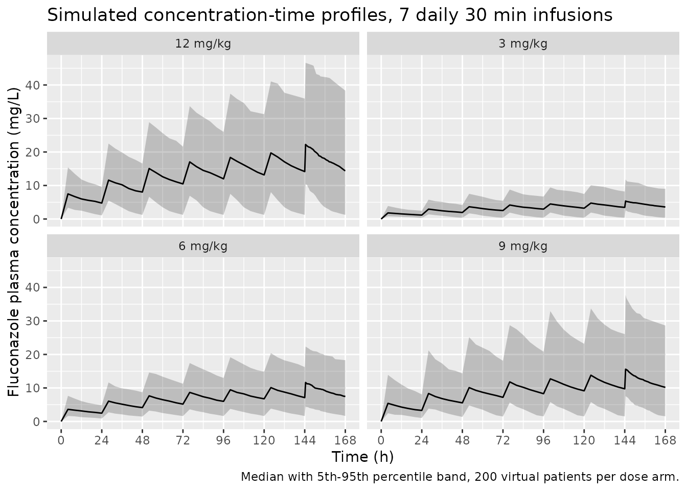
The wide bands are a faithful consequence of the published between-subject variability: 88.5% CV on clearance is unusually large, and the paper’s own Discussion attributes it to the small, heterogeneous cohort.

PKNCA validation

Typical-value NCA against the paper’s printed clearance and volume

Section 3.2 and the Discussion print weight-normalised clearance and volume at specific body weights. Running a single intravenous dose through the packaged model with the random effects zeroed and passing the result through PKNCA should recover exactly those values, because for a one-compartment model CL = Dose/AUC0-inf and Vz = CL/lambda_z = V.

mod_typical <- rxode2::zeroRe(mod)
#> ℹ parameter labels from comments will be replaced by 'label()'

nca_weights <- c(6.0, 58.5, 70.0)

typ_events <- tibble::tibble(id = seq_along(nca_weights), WT = nca_weights) |>
  dplyr::mutate(
    treatment = paste0(format(WT, trim = TRUE), " kg"),
    amt_mg = 6 * WT  # 6 mg/kg single dose; NCA identities are dose-independent
  )

typ_doses <- typ_events |>
  dplyr::mutate(time = 0, evid = 1L, cmt = "central", amt = amt_mg,
                rate = amt_mg / 0.5)

typ_obs <- typ_events |>
  tidyr::crossing(time = c(seq(0, 2, by = 0.05), seq(2.5, 24, by = 0.5),
                           seq(25, 1000, by = 2))) |>
  dplyr::mutate(evid = 0L, cmt = "central", amt = NA_real_, rate = NA_real_)

typ_ev <- dplyr::bind_rows(typ_doses, typ_obs) |>
  dplyr::arrange(id, time, dplyr::desc(evid)) |>
  dplyr::select(id, time, amt, rate, evid, cmt, WT, treatment)

sim_typ <- rxode2::rxSolve(
  mod_typical,
  events = as.data.frame(typ_ev),
  keep = c("WT", "treatment"),
  useLinCmt = FALSE
) |>
  as.data.frame() |>
  dplyr::mutate(id = as.integer(as.character(id)))
#> ℹ omega/sigma items treated as zero: 'etalcl', 'etalvc'
#> Warning: multi-subject simulation without without 'omega'

conc_typ <- sim_typ |>
  dplyr::filter(!is.na(Cc)) |>
  dplyr::select(id, time, Cc, treatment)

conc_typ <- dplyr::bind_rows(
  conc_typ,
  conc_typ |> dplyr::distinct(id, treatment) |>
    dplyr::mutate(time = 0, Cc = 0)
) |>
  dplyr::distinct(id, treatment, time, .keep_all = TRUE) |>
  dplyr::arrange(id, treatment, time)

dose_typ <- typ_doses |>
  dplyr::select(id, time, amt, treatment)

conc_obj <- PKNCA::PKNCAconc(as.data.frame(conc_typ), Cc ~ time | treatment + id)
dose_obj <- PKNCA::PKNCAdose(
  as.data.frame(dose_typ), amt ~ time | treatment + id,
  route = "intravascular", duration = 0.5
)

intervals_typ <- data.frame(
  start = 0, end = Inf,
  cmax = TRUE, tmax = TRUE, aucinf.obs = TRUE,
  half.life = TRUE, cl.obs = TRUE, vz.obs = TRUE
)

nca_typ <- PKNCA::pk.nca(
  PKNCA::PKNCAdata(conc_obj, dose_obj, intervals = intervals_typ)
)

The reference column below is transcribed from the paper: CL/WT of 0.31 mL/min/kg at 58.5 kg and 0.55 mL/min/kg at 6.0 kg (Section 3.2), CL of 1.24 L/h at the 70 kg allometric reference (Table 2), and V/WT of 1.49 L/kg (Section 3.2, with the 70 kg entry taken directly from the Table 2 estimate of 104.07 L).

published <- tibble::tribble(
  ~treatment,  ~cl.obs,                    ~vz.obs,
  "6 kg",      0.55 * 6.0 * 60 / 1000,     1.49 * 6.0,
  "58.5 kg",   0.31 * 58.5 * 60 / 1000,    1.49 * 58.5,
  "70 kg",     1.24,                       104.07
)

cmp <- nlmixr2lib::ncaComparisonTable(
  simulated = nca_typ,
  reference = published,
  by = "treatment",
  units = c(cl.obs = "L/h", vz.obs = "L"),
  tolerance_pct = 20
)

knitr::kable(
  cmp,
  caption = "Simulated NCA from the packaged model versus the clearance and volume values printed by Adamiszak 2025. * marks a >20% difference.",
  digits = 3
)

Simulated NCA from the packaged model versus the clearance and volume values printed by Adamiszak 2025. * marks a >20% difference.

NCA parameter	treatment	Reference	Simulated	% diff
CL/F (L/h)	58.5 kg	1.09	1.08	-0.4%
Vz/F (L)	58.5 kg	87.2	87	-0.2%

# Per-subject identity: for a one-compartment IV model the NCA clearance must
# equal the structural clearance exactly.
cl_nca <- as.data.frame(nca_typ) |>
  dplyr::filter(PPTESTCD == "cl.obs") |>
  dplyr::select(treatment, cl_nca = PPORRES)

cl_struct <- tibble::tibble(
  treatment = paste0(format(nca_weights, trim = TRUE), " kg"),
  cl_struct = allom_cl(nca_weights)
)

identity_check <- dplyr::inner_join(cl_nca, cl_struct, by = "treatment") |>
  dplyr::mutate(rel_diff = abs(cl_nca - cl_struct) / cl_struct)

knitr::kable(identity_check, digits = 5,
             caption = "NCA-derived CL versus the allometric structural CL.")

NCA-derived CL versus the allometric structural CL.

treatment	cl_nca	cl_struct	rel_diff
58.5 kg	1.08384	1.08384	0
6.0 kg	0.19643	0.19643	0
70.0 kg	1.24000	1.24000	0

stopifnot(nrow(identity_check) == 3, all(identity_check$rel_diff < 0.005))

The half-life implied by the model deserves comment. At the 70 kg reference the model gives 58 h, appreciably longer than the roughly 30 h the authors assume in Section 2.4 when they justify sampling the sixth dosing interval. That follows directly from the reported volume, which the Discussion itself flags as about 50% higher than published paediatric and adult values and attributes to the underlying illness, chemotherapy, and hyper-hydration. It is a property of the published estimates, not of this re-implementation.

Steady-state exposure in the virtual cohort

conc_ss <- sim |>
  dplyr::filter(!is.na(Cc), time >= 144) |>
  dplyr::select(id, time, Cc, treatment)

conc_obj_ss <- PKNCA::PKNCAconc(as.data.frame(conc_ss), Cc ~ time | treatment + id)

dose_ss <- events |>
  dplyr::filter(evid == 1, time == 144) |>
  dplyr::select(id, time, amt, treatment)

dose_obj_ss <- PKNCA::PKNCAdose(
  as.data.frame(dose_ss), amt ~ time | treatment + id,
  route = "intravascular", duration = 0.5
)

intervals_ss <- data.frame(
  start = 144, end = 168,
  auclast = TRUE, cmax = TRUE, cmin = TRUE
)

nca_ss <- PKNCA::pk.nca(
  PKNCA::PKNCAdata(conc_obj_ss, dose_obj_ss, intervals = intervals_ss)
)

auc_ss <- as.data.frame(nca_ss) |>
  dplyr::filter(PPTESTCD == "auclast") |>
  dplyr::select(treatment, id, auc_144_168 = PPORRES)

auc_ss |>
  dplyr::group_by(treatment) |>
  dplyr::summarise(
    `Median fAUC (mg*h/L)` = median(0.89 * auc_144_168),
    `5th percentile` = quantile(0.89 * auc_144_168, 0.05),
    `95th percentile` = quantile(0.89 * auc_144_168, 0.95),
    .groups = "drop"
  ) |>
  dplyr::rename("Dose" = treatment) |>
  knitr::kable(
    digits = 1,
    caption = "Simulated free-drug AUC over 144-168 h. The free fraction 0.89 follows Section 2.4 ('the free fraction of FLU was calculated based on the ~11% protein binding')."
  )

Simulated free-drug AUC over 144-168 h. The free fraction 0.89 follows Section 2.4 (‘the free fraction of FLU was calculated based on the ~11% protein binding’).

Dose	Median fAUC (mg*h/L)	5th percentile	95th percentile
12 mg/kg	384.9	100.7	903.2
3 mg/kg	93.9	28.6	213.9
6 mg/kg	199.4	67.2	422.5
9 mg/kg	263.3	87.7	656.0

Probability of target attainment

The exposure identity used for the target-attainment grid

The paper’s target-attainment analysis integrates the free-drug AUC over 144 to 168 h after once-daily 30 min infusions (Section 2.4). For a one-compartment linear model this interval AUC has a closed form. Mass balance over the window gives AUC = (dose_in - (A_end - A_start)) / CL, and evaluating the amounts for n equally spaced infusions of duration Tinf yields

AUC(144, 168) = (D / CL) * (1 - phi * r^n)
  where r   = exp(-tau * CL / V)
        phi = (exp(Tinf * CL / V) - 1) / (Tinf * CL / V)

with tau = 24 h, Tinf = 0.5 h, and n = 7 doses given at 0, 24, …, 144 h. The closed form is validated below against the PKNCA integration of the actual rxode2 solution, subject by subject, before it is used to build the grid.

auc_closed <- function(dose_mg, cl, v, tau = 24, tinf = 0.5, n = 7) {
  k <- cl / v
  r <- exp(-tau * k)
  phi <- (exp(tinf * k) - 1) / (tinf * k)
  (dose_mg / cl) * (1 - phi * r^n)
}

subj_par <- sim |>
  dplyr::group_by(id, treatment) |>
  dplyr::summarise(
    WT = dplyr::first(WT), cl = dplyr::first(cl), vc = dplyr::first(vc),
    .groups = "drop"
  ) |>
  dplyr::left_join(
    events |> dplyr::filter(evid == 1, time == 144) |> dplyr::select(id, amt),
    by = "id"
  ) |>
  dplyr::mutate(auc_formula = auc_closed(amt, cl, vc))

auc_check <- dplyr::inner_join(subj_par, auc_ss, by = c("id", "treatment")) |>
  dplyr::mutate(rel_diff = abs(auc_formula - auc_144_168) / auc_144_168)

sprintf(
  "Closed form vs PKNCA over %d subjects: median |relative difference| %.2e, max %.2e",
  nrow(auc_check), median(auc_check$rel_diff), max(auc_check$rel_diff)
)
#> [1] "Closed form vs PKNCA over 800 subjects: median |relative difference| 1.25e-06, max 3.73e-04"

stopifnot(nrow(auc_check) == length(dose_levels) * n_per_arm,
          max(auc_check$rel_diff) < 0.01)

Reproducing the deposited target-attainment tables

The authors deposited the exact target-attainment percentages behind Figure S10 in their public repository (AUCtoMIC_100_PTA.xlsx and AUCtoMIC_50_PTA.xlsx, sheet “6-60kg per 6kg”). Those percentages are transcribed below and compared against a re-simulation from the packaged model. Following Section 2.4 the grid uses 2500 virtual patients per cell, an MIC of 2 mg/L, a free fraction of 0.89, and the fAUC/MIC targets of 100 and 50, i.e. free AUC over 144 to 168 h of at least 200 and 100 mg*h/L respectively. Because the closed form above was validated against the ODE solution subject by subject, the grid is evaluated from it rather than by re-solving 60 more ODE cohorts.

set.seed(488)

omega_cl <- sqrt(log(1 + 0.8854^2))
omega_v  <- sqrt(log(1 + 0.5585^2))

n_pta <- 2500L  # matches Section 2.4: "2500 virtual patients were simulated"

# Common random numbers: one set of individuals reused across every weight and
# dose cell, matching "accounting for the same individuals among the simulated
# groups" (Section 2.4).
eta_cl <- rnorm(n_pta, 0, omega_cl)
eta_v  <- rnorm(n_pta, 0, omega_v)

pta_cell <- function(wt, mgkg, target_fauc) {
  cl <- allom_cl(wt) * exp(eta_cl)
  v  <- allom_v(wt) * exp(eta_v)
  fauc <- 0.89 * auc_closed(mgkg * wt, cl, v)
  100 * mean(fauc >= target_fauc)
}

pta_weights <- seq(6, 60, by = 6)
pta_doses <- c(3, 6, 9, 12, 15, 18)

pta_grid <- function(target_fauc) {
  tidyr::expand_grid(WT = pta_weights, mgkg = pta_doses) |>
    dplyr::mutate(PTA = mapply(pta_cell, WT, mgkg, target_fauc))
}

pta100 <- pta_grid(200)  # fAUC/MIC >= 100 at MIC = 2 mg/L
pta50 <- pta_grid(100)   # fAUC/MIC >= 50  at MIC = 2 mg/L

# Transcribed from the author deposit, sheet "6-60kg per 6kg".
deposited100 <- tibble::tribble(
  ~WT, ~`3`, ~`6`, ~`9`, ~`12`, ~`15`, ~`18`,
  6,     4,   31,   57,    72,    82,    88,
  12,    6,   38,   66,    79,    88,    91,
  18,    7,   46,   70,    82,    90,    93,
  24,    9,   47,   74,    85,    91,    95,
  30,   10,   52,   77,    87,    93,    96,
  36,   11,   54,   78,    88,    93,    97,
  42,   11,   55,   80,    90,    94,    97,
  48,   11,   58,   82,    90,    95,    97,
  54,   14,   60,   82,    92,    95,    97,
  60,   14,   60,   83,    92,    95,    97
) |>
  tidyr::pivot_longer(-WT, names_to = "mgkg", values_to = "PTA_published") |>
  dplyr::mutate(mgkg = as.numeric(mgkg))

deposited50 <- tibble::tribble(
  ~WT, ~`3`, ~`6`, ~`9`, ~`12`, ~`15`, ~`18`,
  6,    31,   74,   87,    94,    97,    98,
  12,   41,   79,   93,    97,    98,    99,
  18,   45,   83,   93,    98,    99,    99,
  24,   48,   86,   95,    98,    99,    99,
  30,   50,   87,   95,    98,    99,   100,
  36,   54,   88,   97,    98,    99,   100,
  42,   56,   89,   97,    99,    99,   100,
  48,   57,   91,   97,    99,   100,   100,
  54,   59,   91,   97,    99,   100,   100,
  60,   60,   92,   97,    99,   100,   100
) |>
  tidyr::pivot_longer(-WT, names_to = "mgkg", values_to = "PTA_published") |>
  dplyr::mutate(mgkg = as.numeric(mgkg))

pta_cmp <- dplyr::bind_rows(
  dplyr::inner_join(pta100, deposited100, by = c("WT", "mgkg")) |>
    dplyr::mutate(Target = "fAUC/MIC >= 100"),
  dplyr::inner_join(pta50, deposited50, by = c("WT", "mgkg")) |>
    dplyr::mutate(Target = "fAUC/MIC >= 50")
) |>
  dplyr::mutate(diff = PTA - PTA_published)

sprintf(
  "PTA cells compared: %d. Mean absolute difference %.2f percentage points; maximum %.1f.",
  nrow(pta_cmp), mean(abs(pta_cmp$diff)), max(abs(pta_cmp$diff))
)
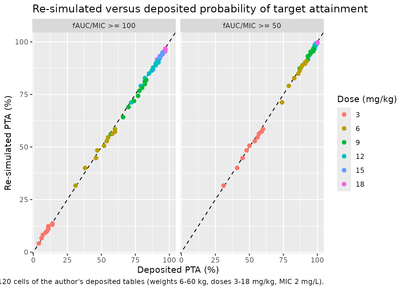
#> [1] "PTA cells compared: 120. Mean absolute difference 0.75 percentage points; maximum 2.8."

# The deposited percentages come from 2500-patient Monte Carlo runs and are
# reported as whole percent, so a few points of disagreement is expected noise.
stopifnot(
  nrow(pta_cmp) == 120,
  mean(abs(pta_cmp$diff)) < 2,
  max(abs(pta_cmp$diff)) <= 4
)

pta100 |>
  dplyr::mutate(PTA = round(PTA)) |>
  tidyr::pivot_wider(names_from = mgkg, values_from = PTA, names_prefix = "dose_") |>
  dplyr::rename(
    "Weight (kg)" = WT,
    "3 mg/kg" = dose_3, "6 mg/kg" = dose_6, "9 mg/kg" = dose_9,
    "12 mg/kg" = dose_12, "15 mg/kg" = dose_15, "18 mg/kg" = dose_18
  ) |>
  knitr::kable(
    caption = "Replicates Figure S10 (top) of Adamiszak 2025: probability of target attainment (%) for fAUC/MIC >= 100 with Candida spp. MIC = 2 mg/L."
  )

Replicates Figure S10 (top) of Adamiszak 2025: probability of target attainment (%) for fAUC/MIC >= 100 with Candida spp. MIC = 2 mg/L.

Weight (kg)	3 mg/kg	6 mg/kg	9 mg/kg	12 mg/kg	15 mg/kg	18 mg/kg
6	4	32	56	71	81	87
12	7	40	64	79	87	92
18	8	45	69	83	90	93
24	9	48	72	85	91	94
30	10	51	74	86	92	95
36	11	53	77	88	93	96
42	12	55	78	89	94	96
48	12	56	80	90	94	96
54	13	57	81	90	95	97
60	14	59	82	91	95	97

pta50 |>
  dplyr::mutate(PTA = round(PTA)) |>
  tidyr::pivot_wider(names_from = mgkg, values_from = PTA, names_prefix = "dose_") |>
  dplyr::rename(
    "Weight (kg)" = WT,
    "3 mg/kg" = dose_3, "6 mg/kg" = dose_6, "9 mg/kg" = dose_9,
    "12 mg/kg" = dose_12, "15 mg/kg" = dose_15, "18 mg/kg" = dose_18
  ) |>
  knitr::kable(
    caption = "Replicates Figure S10 (bottom) of Adamiszak 2025: probability of target attainment (%) for fAUC/MIC >= 50 with Candida spp. MIC = 2 mg/L."
  )

Replicates Figure S10 (bottom) of Adamiszak 2025: probability of target attainment (%) for fAUC/MIC >= 50 with Candida spp. MIC = 2 mg/L.

Weight (kg)	3 mg/kg	6 mg/kg	9 mg/kg	12 mg/kg	15 mg/kg	18 mg/kg
6	32	71	87	93	96	98
12	40	79	92	96	98	99
18	45	83	93	97	99	99
24	48	85	94	97	99	99
30	51	86	95	98	99	99
36	53	88	96	98	99	100
42	55	89	96	99	99	100
48	56	90	96	99	99	100
54	57	90	97	99	99	100
60	59	91	97	99	99	100

pta_cmp |>
  ggplot(aes(PTA_published, PTA, colour = factor(mgkg))) +
  geom_abline(slope = 1, intercept = 0, linetype = "dashed") +
  geom_point(size = 2) +
  facet_wrap(~Target) +
  labs(
    x = "Deposited PTA (%)", y = "Re-simulated PTA (%)",
    colour = "Dose (mg/kg)",
    title = "Re-simulated versus deposited probability of target attainment",
    caption = "All 120 cells of the author's deposited tables (weights 6-60 kg, doses 3-18 mg/kg, MIC 2 mg/L)."
  )

The paper’s dosing conclusions

pta100 |>
  dplyr::filter(PTA >= 90) |>
  dplyr::arrange(mgkg, WT) |>
  dplyr::rename("Weight (kg)" = WT, "Dose (mg/kg)" = mgkg, "PTA (%)" = PTA) |>
  dplyr::mutate(`PTA (%)` = round(`PTA (%)`)) |>
  knitr::kable(
    caption = "Cells reaching the 90% acceptability threshold for fAUC/MIC >= 100 at MIC = 2 mg/L."
  )

Cells reaching the 90% acceptability threshold for fAUC/MIC >= 100 at MIC = 2 mg/L.

Weight (kg)	Dose (mg/kg)	PTA (%)
54	12	90
60	12	91
24	15	91
30	15	92
36	15	93
42	15	94
48	15	94
54	15	95
60	15	95
12	18	92
18	18	93
24	18	94
30	18	95
36	18	96
42	18	96
48	18	96
54	18	97
60	18	97

Within the SmPC range (3 to 12 mg/kg) only the 12 mg/kg dose in the heaviest children reaches the 90% threshold for the stringent fAUC/MIC >= 100 target, which is exactly the paper’s Section 3.3 conclusion: “already registered FLU dosages exceed the assumed 90% of PTA in the case of 48-60 kg patients treated with 12 mg/kg FLU dose.”

pta50 |>
  dplyr::filter(mgkg %in% c(9, 12)) |>
  dplyr::group_by(mgkg) |>
  dplyr::summarise(
    `Minimum PTA across 6-60 kg (%)` = round(min(PTA)),
    .groups = "drop"
  ) |>
  dplyr::rename("Dose (mg/kg)" = mgkg) |>
  knitr::kable(
    caption = "For the less rigorous fAUC/MIC >= 50 target, the higher SmPC doses clear 90% PTA at every simulated weight (Section 3.3)."
  )

For the less rigorous fAUC/MIC >= 50 target, the higher SmPC doses clear 90% PTA at every simulated weight (Section 3.3).

Dose (mg/kg)	Minimum PTA across 6-60 kg (%)
9	87
12	93

Doses below 6 mg/kg never approach the acceptability threshold at either target, reproducing the paper’s central finding that registered fluconazole doses under 6 mg/kg leave hemato-oncologic children subtherapeutic.

Assumptions and deviations

• Weight distribution. The paper does not publish the weight distribution used for its Monte Carlo simulations, only the 6 to 60 kg grid of the target-attainment figures. The virtual cohort in the “Virtual cohort” section draws weights log-uniformly over the observed 6.0 to 58.5 kg range; the target-attainment grid instead fixes weight at each grid point exactly as Figure S10 does, so no distributional assumption enters the PTA comparison.
• Dose timing for the 144 to 168 h window. Section 2.4 states that the free AUC was taken “after the 6th dose (between 144 and 168 h)”. Taken literally these two statements are inconsistent if the first dose is at time 0 (the sixth dose would then start the 120 to 144 h interval). The explicit window, 144 to 168 h, was used, with once-daily doses at 0, 24, …, 144 h. This is the interpretation that reproduces the deposited target-attainment percentages, as the comparison above shows.
• Free fraction. Section 2.4 says the free fraction was “calculated based on the ~11% protein binding in the SmPC”, which is taken here as fu = 0.89. The authors state elsewhere that binding is reported as 11-12%; 0.88 instead of 0.89 shifts every target-attainment cell by well under one percentage point.
• Residual error in the target-attainment analysis. Exposure targets are evaluated on the model-predicted individual AUC, which carries between-subject variability but not residual error. This matches the paper, whose target is defined on fAUC rather than on a measured concentration.
• Closed-form interval AUC. The target-attainment grid is evaluated from the analytic interval-AUC expression rather than from 60 additional rxode2 cohorts. The expression is not an assumption: it is validated in the “exposure identity” chunk against the PKNCA integration of the actual ODE solution for all 800 simulated subjects, and the check fails the build if the agreement is worse than 1%.
• Covariates screened but not retained. Age, eGFR, sex, and serum creatinine were screened by stepwise covariate modelling and by the mlcov package but do not appear in the final model, and the paper publishes no coefficients for them (only median-split summaries and post hoc regressions in Figures 2 and 3). They are recorded in the model file’s covariatesDataExcluded list so the provenance of the covariate screen is preserved without declaring covariates the model never uses.
• Infusion duration. Patients in the study received 0.5 or 1 h infusions (Section 3.1), but the simulations in Section 2.4 specify a 30 min infusion; 30 min is used here. For a drug with a multi-day half-life the interval AUC is insensitive to this choice.
• No independent NCA reference. The paper reports no observed NCA table, so the “Comparison against published NCA” table is built from the clearance and volume values the paper prints in Section 3.2 and Table 2, which PKNCA must recover exactly for a one-compartment intravenous model.