Ivermectin lung exposure minimal PBPK (Jermain 2020)
Source:vignettes/articles/Jermain_2020_ivermectin_pbpk.Rmd
Jermain_2020_ivermectin_pbpk.RmdModel and source
Jermain et al. (2020) built a minimal physiologically-based pharmacokinetic (mPBPK) model to ask whether oral ivermectin, repurposed against SARS-CoV-2, reaches lung concentrations near its in vitro IC50 of 1750 ng/mL. The model has a transit compartment and an absorption compartment feeding plasma, a lung compartment that receives the whole cardiac output, and a lumped rest-of-body (“Other”) compartment that receives a fraction of it. Both tissues are perfusion-rate-limited.
mod <- readModelDb("Jermain_2020_ivermectin_pbpk")
ui <- rxode2::rxode(mod)- Citation: Jermain B, Hanafin PO, Cao Y, Lifschitz A, Lanusse C, Rao GG. Development of a Minimal Physiologically-Based Pharmacokinetic Model to Simulate Lung Exposure in Humans Following Oral Administration of Ivermectin for COVID-19 Drug Repurposing. J Pharm Sci. 2020;109(12):3574-3578. doi:10.1016/j.xphs.2020.08.024.
- Article: https://doi.org/10.1016/j.xphs.2020.08.024
- PubMed Central: https://www.ncbi.nlm.nih.gov/pmc/articles/PMC7473010/
PBPK (minimal, four-compartment; Phoenix WinNonlin 8.2). Oral ivermectin disposition in adults with a transit-delayed first-order absorption, a plasma compartment, a lung compartment perfused by the full cardiac output and a lumped rest-of-body (Other) compartment perfused by a fraction of the cardiac output (Jermain et al. 2020, J Pharm Sci 109:3574). Tissue uptake is perfusion-rate-limited. Plasma volume, lung volume, cardiac output and the remaining volume are fixed physiological values; the lung partition coefficient was fixed from the lung-to-plasma AUC ratio in calves given subcutaneous ivermectin; ka, CL/F, the Other partition coefficient, the fraction of cardiac output and the transit rate were fitted to a simulated geometric-mean plasma profile after a 15 mg oral dose. Clearance and the partition coefficients are apparent (divided by oral bioavailability F). The model carries no between-subject variability and was built to predict total ivermectin concentrations in lung tissue after single oral doses for COVID-19 repurposing.
Population
The human part of the model was not fitted to individual data. The authors took the population PK model of a phase 1 study in 18 healthy volunteers given 0.2 mg/kg oral ivermectin (El-Tahtawy et al., reference 13 of the paper), simulated its geometric-mean plasma profile for the study-average dose of 15 mg without between-subject or residual variability, and fitted the five free mPBPK parameters to that profile in Phoenix WinNonlin 8.2 (Methods, “Ivermectin Pharmacokinetic Data” and “Parameters”).
The lung partition coefficient came from a different species: it is the ratio of lung to plasma AUC in Holstein calves given 0.2 mg/kg subcutaneous ivermectin (Lifschitz et al., reference 12), assumed to be species-independent because plasma protein binding is similarly high in cattle and humans. Physiological volumes and cardiac output are population averages for adults (references 14 and 15). No covariates are carried.
Source trace
| Quantity | Model name | Value | Source |
|---|---|---|---|
| Absorption rate constant | lka |
0.14 1/h | Table 1 (CV 2.52%) |
| Apparent plasma clearance CLp/F | lcl |
10.85 L/h | Table 1 (CV 3.78%) |
| Apparent Other partition coefficient Kp,other/F | lkp_other |
17.32 | Table 1 (CV 5.6%) |
| Fraction of cardiac output to Other | fq_other |
0.08 | Table 1 (CV 1.18%) |
| Transit rate constant | lktr |
0.36 1/h | Table 1 (CV 3.09%) |
| Apparent lung partition coefficient Kp,lung/F | lkp_lung |
2.68 (fixed) | Table 1, footnote a; calf AUC ratio (Methods) |
| Plasma volume | lvc |
3 L (fixed) | Table 1, footnote a (ref 15) |
| Lung volume | lv_lung |
1.3 L (fixed) | Table 1, footnote a (ref 14) |
| Remaining volume | lv_other |
65.7 L (fixed) | Table 1, footnote a |
| Cardiac output | q_co |
282 L/h (fixed) | Table 1, footnote a (ref 15) |
| Residual error, plasma and lung |
propSd, propSd_Clung
|
20% (fixed) | Methods, “Human Lung Exposure Simulation” |
| Transit and absorption ODEs |
depot, transit1
|
– | page 3576, equations for a0 and Absorption |
| Plasma ODE | central |
– | page 3576, plasma equation (full-width) |
| Lung and Other ODEs |
lung, other
|
– | page 3576, right column |
| Model schematic | – | – | Figure 1 |
Typical-value simulation of the fitted 15 mg profile (Figure 2)
Figure 2 of the paper overlays the mPBPK fit on the simulated geometric-mean plasma profile after 15 mg. The published points are not tabulated, so only the model curve is reproduced here.
mod_typ <- rxode2::zeroRe(mod)
#> Warning: No omega parameters in the model

# The model has two error endpoints (plasma and lung), so each observation row
# names its endpoint with dvid; both Cc and Clung come back as columns.
make_events <- function(dose, times, n = 1) {
  dplyr::bind_rows(
    data.frame(id = seq_len(n), time = 0, amt = dose, evid = 1L,
               cmt = "depot", dvid = NA_integer_),
    expand.grid(id = seq_len(n), time = times) |>
      dplyr::mutate(amt = 0, evid = 0L, cmt = NA_character_, dvid = 1L)
  ) |>
    dplyr::arrange(id, time, dplyr::desc(evid))
}

sim15 <- as.data.frame(rxode2::rxSolve(mod_typ, make_events(15, seq(0, 72, by = 0.1))))

ggplot(sim15, aes(time, Cc)) +
  geom_line(colour = "steelblue") +
  labs(x = "Time after dose (h)", y = "Plasma ivermectin (ng/mL)",
       title = "Replicates Figure 2 of Jermain 2020 (model curve)",
       caption = "Single 15 mg oral dose, typical values.")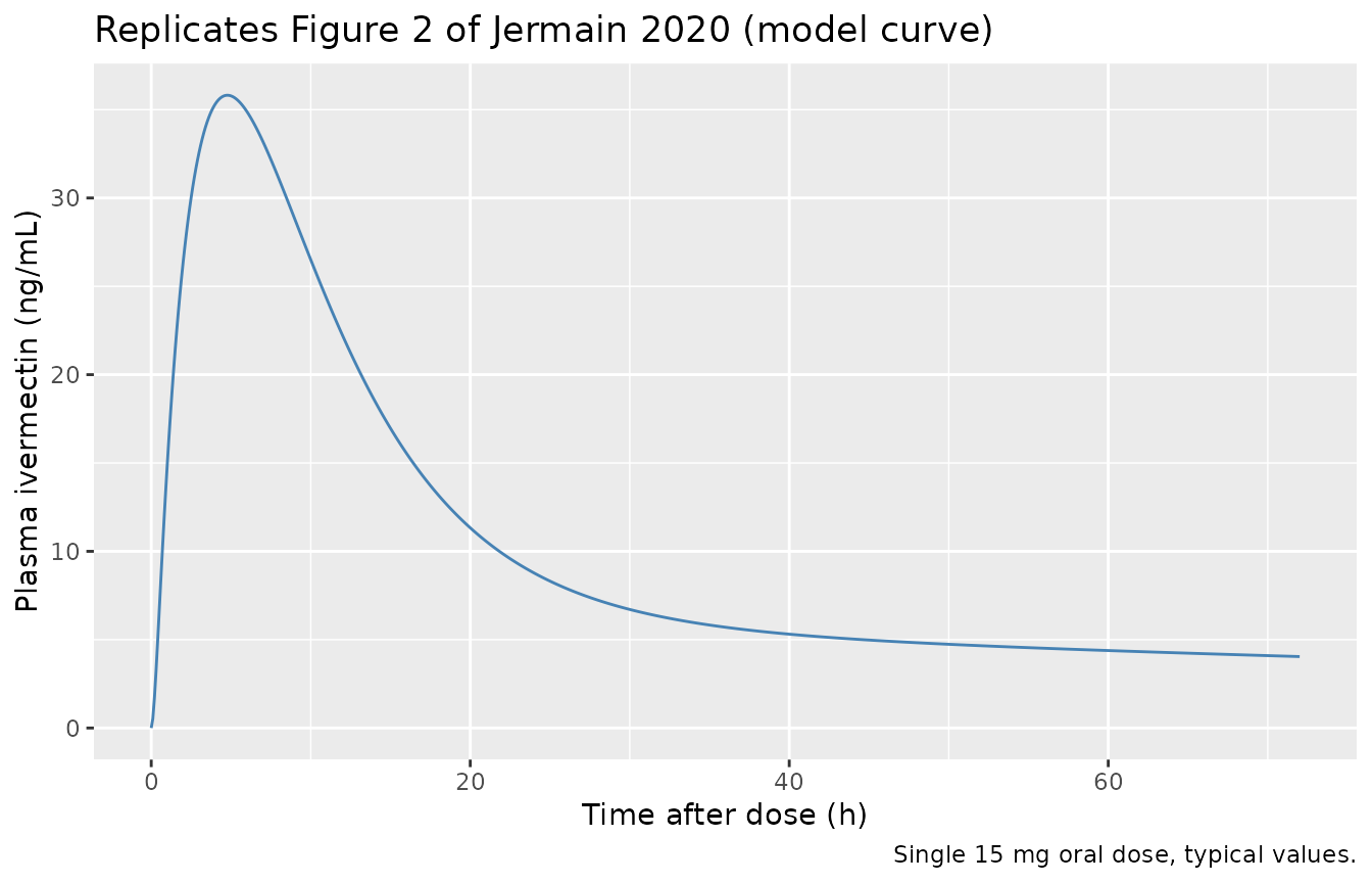
Lung and plasma exposure after 12, 30 and 120 mg (Figure 3, Figure S1)
The authors simulated 1000 subjects per dose on a 0.1 h grid with an assumed 20% residual error and no between-subject variability, and plotted the median and 95% interval. A cohort of 200 per dose is used here.
rxode2::rxSetSeed(20200904)
doses <- c(12, 30, 120)
times <- seq(0, 72, by = 0.1)

sim_sto <- dplyr::bind_rows(lapply(doses, function(d) {
  as.data.frame(rxode2::rxSolve(mod, make_events(d, times, n = 200))) |>
    dplyr::mutate(dose = d)
}))
#> Warning: multi-subject simulation without without 'omega'
#> Warning: multi-subject simulation without without 'omega'
#> Warning: multi-subject simulation without without 'omega'

band <- sim_sto |>
  tidyr::pivot_longer(c(Cc, Clung), names_to = "matrix", values_to = "conc") |>
  dplyr::mutate(matrix = ifelse(matrix == "Cc", "Plasma", "Lung")) |>
  dplyr::group_by(dose, matrix, time) |>
  dplyr::summarise(
    median = stats::median(conc),
    lo = stats::quantile(conc, 0.025),
    hi = stats::quantile(conc, 0.975),
    .groups = "drop"
  )

ggplot(band, aes(time, median, colour = matrix, fill = matrix)) +
  geom_ribbon(aes(ymin = lo, ymax = hi), alpha = 0.2, colour = NA) +
  geom_line() +
  geom_hline(yintercept = 1750, linetype = "dashed") +
  facet_wrap(~ paste(dose, "mg"), scales = "free_y") +
  labs(x = "Time after dose (h)", y = "Ivermectin (ng/mL)",
       colour = NULL, fill = NULL,
       title = "Replicates Figure 3 (120 mg) and Figure S1 (12, 30 mg)",
       caption = "Median and 95% interval of 200 simulated subjects; dashed line = in vitro IC50.")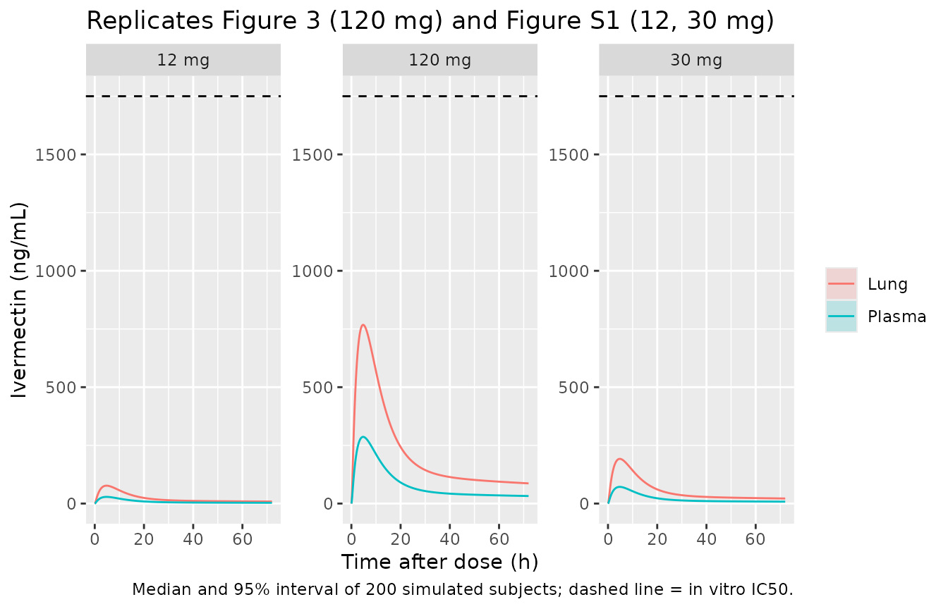
The stochastic median tracks the typical-value profile, since the only variability in the model is residual error:
sim120_typ <- as.data.frame(rxode2::rxSolve(mod_typ, make_events(120, times)))
med120 <- band |>
  dplyr::filter(dose == 120) |>
  dplyr::group_by(matrix) |>
  dplyr::summarise(cmax_median = max(median), .groups = "drop")
med120
#> # A tibble: 2 × 2
#>   matrix cmax_median
#>   <chr>        <dbl>
#> 1 Lung          768.
#> 2 Plasma        287.

stopifnot(
  abs(med120$cmax_median[med120$matrix == "Plasma"] / max(sim120_typ$Cc) - 1) < 0.1,
  abs(med120$cmax_median[med120$matrix == "Lung"] / max(sim120_typ$Clung) - 1) < 0.1
)
PKNCA validation
NCA is run on the typical-value profiles for each dose, separately for plasma and lung, over a long enough window (0-2000 h) that the extrapolated AUC is negligible.
nca_times <- sort(unique(c(seq(0, 24, by = 0.1), seq(25, 2000, by = 5))))
sim_nca <- dplyr::bind_rows(lapply(doses, function(d) {
  as.data.frame(rxode2::rxSolve(mod_typ, make_events(d, nca_times))) |>
    dplyr::mutate(id = 1L, treatment = paste(d, "mg"), dose = d)
}))

run_nca <- function(conc_col) {
  conc_df <- sim_nca |>
    dplyr::transmute(id, treatment, time, conc = .data[[conc_col]]) |>
    dplyr::filter(!is.na(conc))
  dose_df <- sim_nca |>
    dplyr::distinct(id, treatment, dose) |>
    dplyr::mutate(time = 0)
  res <- PKNCA::pk.nca(PKNCA::PKNCAdata(
    PKNCA::PKNCAconc(conc_df, conc ~ time | treatment + id),
    PKNCA::PKNCAdose(dose_df, dose ~ time | treatment + id),
    intervals = data.frame(start = 0, end = Inf, cmax = TRUE, tmax = TRUE,
                           aucinf.obs = TRUE, half.life = TRUE)
  ))
  as.data.frame(res)
}

nca_plasma <- run_nca("Cc") |> dplyr::mutate(matrix = "Plasma")
nca_lung <- run_nca("Clung") |> dplyr::mutate(matrix = "Lung")

nca_all <- dplyr::bind_rows(nca_plasma, nca_lung) |>
  dplyr::filter(PPTESTCD %in% c("cmax", "tmax", "aucinf.obs", "half.life")) |>
  dplyr::select(matrix, treatment, PPTESTCD, PPORRES) |>
  tidyr::pivot_wider(names_from = PPTESTCD, values_from = PPORRES)

nca_all |>
  dplyr::rename(
    "Matrix" = matrix, "Dose" = treatment, "Cmax (ng/mL)" = cmax,
    "Tmax (h)" = tmax, "AUC0-inf (h*ng/mL)" = aucinf.obs, "t1/2 (h)" = half.life
  ) |>
knitr::kable(digits = 2, caption = "Typical-value NCA of plasma and lung.")| Matrix | Dose | Cmax (ng/mL) | Tmax (h) | t1/2 (h) | AUC0-inf (h*ng/mL) |
|---|---|---|---|---|---|
| Plasma | 12 mg | 28.65 | 4.8 | 107.76 | 1106.47 |
| Plasma | 120 mg | 286.53 | 4.8 | 107.76 | 11064.70 |
| Plasma | 30 mg | 71.63 | 4.8 | 107.76 | 2766.17 |
| Lung | 12 mg | 76.79 | 4.8 | 107.76 | 2965.33 |
| Lung | 120 mg | 767.90 | 4.8 | 107.76 | 29653.43 |
| Lung | 30 mg | 191.98 | 4.8 | 107.76 | 7413.34 |
Two exact identities follow from the model structure and check that the ODEs were transcribed with the right flows. First, dose over AUC in plasma recovers CLp/F. Second, because the lung is perfused by the full cardiac output in and out, its AUC is exactly Kp,lung/F times the plasma AUC; that ratio is how the authors defined Kp,lung/F from the calf data.
auc_p <- nca_plasma |> dplyr::filter(PPTESTCD == "aucinf.obs") |> dplyr::arrange(treatment)
auc_l <- nca_lung |> dplyr::filter(PPTESTCD == "aucinf.obs") |> dplyr::arrange(treatment)
dose_by_trt <- as.numeric(sub(" mg", "", auc_p$treatment))

cl_recovered <- 1000 * dose_by_trt / auc_p$PPORRES   # mg / (h*ng/mL) -> L/h
ratio_lung <- auc_l$PPORRES / auc_p$PPORRES
data.frame(treatment = auc_p$treatment, cl_recovered, ratio_lung)
#>   treatment cl_recovered ratio_lung
#> 1     12 mg     10.84535   2.680004
#> 2    120 mg     10.84530   2.680003
#> 3     30 mg     10.84533   2.680003

stopifnot(
  all(abs(cl_recovered / 10.85 - 1) < 0.01),
  all(abs(ratio_lung / 2.68 - 1) < 0.01)
)
Comparison against the published 120 mg peak
The paper reports the maximum simulated concentration after 120 mg as 288 ng/mL in plasma and 772 ng/mL in lung, both at 5.1 h (Results, “Human Lung Exposure Simulation”). Those values are read from the median of the authors’ stochastic simulation, which for a model whose only variability is residual error sits on the typical-value profile.
simulated <- nca_all |>
  dplyr::filter(treatment == "120 mg") |>
  dplyr::transmute(group = matrix, cmax, tmax)

published <- data.frame(
  group = c("Plasma", "Lung"),
  cmax = c(288, 772),
  tmax = c(5.1, 5.1)
)

cmp <- nlmixr2lib::ncaComparisonTable(
  simulated = simulated,
  reference = published,
  by = "group",
  tolerance_pct = 20
)
knitr::kable(cmp, caption = "Simulated typical-value 120 mg peak versus Jermain 2020. * marks a difference greater than 20%.")| NCA parameter | group | Reference | Simulated | % diff |
|---|---|---|---|---|
| Cmax | Plasma | 288 | 287 | -0.5% |
| Cmax | Lung | 772 | 768 | -0.5% |
| Tmax | Plasma | 5.1 | 4.8 | -5.9% |
| Tmax | Lung | 5.1 | 4.8 | -5.9% |
typ_cmax <- setNames(simulated$cmax, simulated$group)
stopifnot(
  abs(typ_cmax[["Plasma"]] / 288 - 1) < 0.05,
  abs(typ_cmax[["Lung"]] / 772 - 1) < 0.05
)
The simulated peaks agree with the paper to within about 1%, and the simulated Tmax (about 4.8 h) is within 0.3 h of the published 5.1 h; the published value is the peak of a median over noisy stochastic profiles, which shifts it slightly. Neither dose reaches the 1750 ng/mL in vitro IC50 in lung, matching the paper’s conclusion.
Assumptions and deviations
-
Ka*Doseread asKa*Absorption. The printed absorption and plasma equations (page 3576) write the absorption flux asKa*Dose. Taken literally that is a constant input that never stops and drives the Absorption amount negative. Figure 1 draws the flux from the Absorption compartment to Plasma with rate Ka, and the text calls Ka a first-order absorption rate constant, so the flux is encoded aska * transit1(the Absorption amount). With that reading the model reproduces the published 120 mg plasma and lung peaks to within about 1%. -
Compartment naming. The paper’s transit compartment
a0(which receives the dose) isdepot, and its Absorption compartment istransit1, so the chain reads depot –ktr–> transit1 –ka–> central. - Residual error. The paper used an “assumed 20% RUV” of unstated form for its lung-exposure simulations and does not say whether it applied the same error to lung. It is encoded as a fixed 20% proportional error on both the plasma and the lung output. It was not estimated; the fit itself was to a noise-free profile.
- No between-subject variability. None was estimated or used by the authors, so none is encoded; stochastic simulations vary only by residual error.
-
Apparent (F-scaled) parameters. CLp/F, Kp,lung/F
and Kp,other/F are used exactly as tabulated. Bioavailability is not
separated out, so the dose is given into
depotwith F = 1. -
Cardiac-output topology. As printed, plasma loses
flow to lung at the full cardiac output and to the Other compartment at
Fraction * Qcoin parallel, so the total flow out of plasma is(1 + Fraction) * Qco. That is the published equation set and it is reproduced as written. - Figure 2 data. The simulated geometric-mean plasma concentrations the model was fitted to are shown only graphically; they were not digitised, and the Figure 2 replicate shows the model curve only.
- Supplement. The supplementary material (calf lung and plasma data, Table S1, and the 12 and 30 mg simulations, Figure S1) holds no model parameters; the 12 and 30 mg panels above are simulated from the Table 1 parameters.