Drug A, anti-psoriatic (Zhang 2025)
Source:vignettes/articles/Zhang_2025_drugA.Rmd
Zhang_2025_drugA.RmdModel and source
ui <- rxode2::rxode(readModelDb("Zhang_2025_drugA"))- Citation: Zhang X, Xiao Y, Wu J, Marshall S, Zhou X. Pharmacometric Model-Based Sample Size Allocation for a Region of Interest in a Multi-Regional Phase 2 Trial: A Case Study of an Anti-Psoriatic Drug. CPT Pharmacometrics Syst Pharmacol. 2025;14(10):1673-1681. doi:10.1002/psp4.70090. Parameter values from Table S1; structural equations and variance terms from the Data S4 NONMEM control streams.
- Article: https://doi.org/10.1002/psp4.70090
- Supplement (Table S1, parameter values): https://doi.org/10.1002/psp4.70090 Supporting Information, Table S1
- Supplement (Data S4, NONMEM control streams): https://doi.org/10.1002/psp4.70090 Supporting Information, Data S4
Zhang 2025 is a trial-design paper: its subject is how much of a 175-subject multi-regional Phase 2 dose-ranging trial should be allocated to a region of interest (“Region X”) so that a clinically relevant inter-regional difference in response can be detected. Every number in it comes from simulations of a concrete, fully parameterised dose-exposure-response (D-E-R) model, and the supplement publishes that model in full. This vignette extracts and validates the model itself, not the sample-size methodology.
The structure is a two-compartment PK model with first-order subcutaneous absorption and parallel linear and Michaelis-Menten elimination, feeding an effect (“signaling”) compartment, which in turn inhibits plaque formation in an indirect-response model of the Psoriasis Area and Severity Index (PASI). A placebo effect multiplies the PASI degradation rate and decays exponentially from its maximum at time zero.
Population
The trial simulated by Zhang 2025 enrols approximately 175 adults with plaque psoriasis, randomised 1:1:1:1:1 to Drug A 70, 140 or 210 mg subcutaneously on day 1 and at weeks 1, 2, 4, 6, 8 and 10; Drug A 280 mg on day 1 and at weeks 4 and 8; or placebo (Methods 2.1). The primary endpoint is the percentage improvement from baseline in PASI at week 12.
This is a simulation model rather than a fit to Phase 2 data. The underlying D-E-R model was developed on Phase 1 data for Drug A and carried into this paper “with minor adjustments to parameter values” (Methods 2.2), so the paper reports no fitted-cohort demographics. The typical baseline PASI of 13.5 (Table S1) is the only population characteristic the model itself carries.
pop <- ui$population
str(pop, max.level = 1)
#> List of 9
#>  $ species      : chr "human"
#>  $ n_subjects   : int 175
#>  $ n_studies    : int 1
#>  $ age_range    : chr "not reported (adult psoriasis population)"
#>  $ weight_range : chr "not reported"
#>  $ disease_state: chr "moderate-to-severe plaque psoriasis"
#>  $ dose_range   : chr "Drug A 70, 140 or 210 mg SC at day 1 and weeks 1, 2, 4, 6, 8 and 10; or 280 mg SC at day 1 and weeks 4 and 8; o"| __truncated__
#>  $ regions      : chr "multi-regional; a designated 'Region X' (China, per the Data S4 code comments) versus the rest of the world"
#>  $ notes        : chr "This is a SIMULATION model, not a fit to the Phase 2 data. The N = 175 is the planned size of the hypothetical "| __truncated__
What “Drug A” is, and what “Region X” is
Both are anonymised in the article, and both are recoverable from material the authors themselves published:
-
Drug A is brodalumab. The D-E-R model is cited to
refs 10 and 11, which are Salinger 2014
(
doi:10.1002/cpdd.103, a semi-mechanistic PK/PD model of brodalumab) and Papp 2012 (anti-IL-17-receptor antibody AMG 827, the development code for brodalumab). The parameter values here are the authors’ adjusted set for a hypothetical trial rather than a brodalumab fit, so the model is registered under the paper’s own compound label. The registry’s existingTimmermann_2019_brodalumabis a PK-only model, so this is not a duplicate: it adds the PASI PD layer, the placebo model and the regional covariate. -
Region X is China. The article body says only
“Region X”. The Data S4 R code comments name it:
n_cnis “sample size for cn (Region X)”, and the dataset-construction step adds a “label for Chinese and ROW populations (POP=2 is Region X, POP=1 is non-Region X)”. The covariate is therefore registered as the canonicalREGION_CHINA, with this provenance recorded ininst/references/covariate-columns.md.
Source trace
The per-parameter origin is recorded as an in-file comment next to
each ini() entry in
inst/modeldb/specificDrugs/Zhang_2025_drugA.R. The table
below collects them in one place. Table S1 and the Data S4 control
streams agree on every fixed effect; where they disagree on a
unit or a scale, the resolution is noted.
| Equation / parameter | Value | Source location |
|---|---|---|
lkel |
0.0724 /day | Table S1 Kel; Data S4 PK $THETA(1)
FIX |
lvc |
3.9 L | Table S1 V; Data S4 PK $THETA(2) FIX |
lvmax |
7.4 mg/day | Table S1 Vmax; Data S4 PK $THETA(3)
FIX |
lkm |
0.01 ug/mL | Table S1 Km; Data S4 PK $THETA(4) FIX |
lka |
0.255 /day | Table S1 KA; Data S4 PK $THETA(5) FIX |
lk12 / lk21
|
0.26 / 0.351 /day | Table S1 K12 / K21; Data S4 PK
$THETA(6) / $THETA(7) FIX |
lfdepot |
0.576 | Table S1 F1 (57.6%); Data S4 PK $THETA(8)
FIX |
lrbase |
13.5 PASI | Table S1 BL; Data S4 PD $THETA(1)
|
lksyn |
0.862 PASI/day | Table S1 Ksyn; Data S4 PD $THETA(2)
|
limax |
1 (fixed) | Table S1 Imax; Data S4 PD $THETA(3) “1
FIX” |
lic50 |
2.86 ug/mL | Table S1 IC50; Data S4 PD $THETA(4)
|
lpmax |
0.439 | Table S1 PBOmax; Data S4 PD $THETA(5)
|
lkpl |
0.0372 /day | Table S1 KPBO; Data S4 PD $THETA(6)
|
lke0 |
0.0469 /day | Table S1 Keo; Data S4 PD $THETA(7)
(K50) |
e_region_china_ic50 |
2.6 (fixed) | Data S4 PD $THETA(8) COV_CN, set to
COV_CN_VALUE_PD <- 2.6; Table 1 and Figure 1
caption |
| IIV (6 etas) | see below | Data S4 $OMEGA; each variance square-roots to the %CV
in Table S1 |
| Residual error | see below | Data S4 $SIGMA (variances); see the erratum note |
d/dt(depot), d/dt(central),
d/dt(peripheral1)
|
n/a | Data S4 $DES (both PK and PD streams) |
d/dt(pasi), pasi(0) <- rbase
|
n/a | Data S4 PD $DES DADT(4) and
$PK A_0(4) = BL
|
d/dt(effect), ve <- kel * vc / ke0
|
n/a | Data S4 PD $DES DADT(5) and
$PK V5 = K25*V2/K50, K25 = K
|
ksyn, kdegx
|
n/a | Data S4 PD $DES KSYN and
KDEGX lines |
ui$iniDf |>
  dplyr::mutate(
    estimate = ifelse(is.na(est), NA_real_, est),
    scale = ifelse(is.na(neta1), "theta", "omega (variance)")
  ) |>
  dplyr::select(name, estimate, fix, scale, label) |>
  dplyr::rename(
    "Parameter" = name, "Estimate (transformed scale)" = estimate,
    "Fixed?" = fix, "Scale" = scale, "Label" = label
  ) |>
knitr::kable(digits = 5, caption = "ini() as packaged.")| Parameter | Estimate (transformed scale) | Fixed? | Scale | Label |
|---|---|---|---|---|
| lkel | -2.62555 | TRUE | theta | First-order elimination rate constant from central (1/day) |
| lvc | 1.36098 | TRUE | theta | Central compartment volume (L) |
| lvmax | 2.00148 | TRUE | theta | Maximum rate of Michaelis-Menten elimination (mg/day) |
| lkm | -4.60517 | TRUE | theta | Concentration at half-maximal nonlinear elimination (ug/mL) |
| lka | -1.36649 | TRUE | theta | First-order absorption rate constant (1/day) |
| lk12 | -1.34707 | TRUE | theta | Central-to-peripheral rate constant (1/day) |
| lk21 | -1.04697 | TRUE | theta | Peripheral-to-central rate constant (1/day) |
| lfdepot | -0.55165 | TRUE | theta | Subcutaneous bioavailability (fraction) |
| lrbase | 2.60269 | FALSE | theta | Baseline PASI score (PASI units) |
| lksyn | -0.14850 | FALSE | theta | Zero-order rate of plaque formation, ksyn0 (PASI units/day) |
| limax | 0.00000 | TRUE | theta | Maximum fractional inhibition of plaque formation (unitless) |
| lic50 | 1.05082 | FALSE | theta | Effect-compartment concentration at half-maximal inhibition (ug/mL) |
| lpmax | -0.82326 | FALSE | theta | Maximum fractional increase of the PASI degradation rate by placebo (unitless) |
| lkpl | -3.29145 | FALSE | theta | Decay rate constant of the placebo effect (1/day) |
| lke0 | -3.05974 | FALSE | theta | Effect-compartment (signaling) equilibration rate constant (1/day) |
| e_region_china_ic50 | 2.60000 | TRUE | theta | Ratio of IC50 in Region X patients to IC50 in typical patients (unitless) |
| propSd | 0.51800 | TRUE | theta | Proportional residual error for drug concentration (fraction) |
| addSd | 0.30000 | TRUE | theta | Additive residual error for drug concentration (ug/mL) |
| propSd_pasi | 0.06360 | FALSE | theta | Proportional residual error for PASI score (fraction) |
| addSd_pasi | 1.14500 | FALSE | theta | Additive residual error for PASI score (PASI units) |
| etalvc | 0.08410 | TRUE | omega (variance) | NA |
| etalka | 0.56400 | TRUE | omega (variance) | NA |
| etalvmax | 0.09920 | TRUE | omega (variance) | NA |
| etalrbase | 0.04666 | FALSE | omega (variance) | NA |
| etalic50 | 1.84960 | FALSE | omega (variance) | NA |
| etalke0 | 0.32718 | FALSE | omega (variance) | NA |
Erratum: the PK additive residual in Table S1 is a variance, not an SD
Both endpoints use Y = IPRED * (1 + EPS(1)) + EPS(2), so
the $SIGMA entries are variances. Three of the four rows
confirm it: sqrt(0.2683) = 0.518 is exactly the 51.8% CV
Table S1 states for the PK proportional term,
sqrt(0.00404496) = 0.0636 is its stated 6.36%, and
sqrt(1.31) = 1.145 is its stated 1.145 PASI units. The
fourth row, the PK additive term, is reported by Table S1 as “SD (ug/mL)
0.09” - but 0.09 is the $SIGMA entry, i.e. the variance.
Three consistent rows falsify the fourth: the true PK
additive SD is sqrt(0.09) = 0.3 ug/mL, and the model file
uses 0.3.
tibble::tribble(
  ~term,                      ~sigma,     ~sqrt_sigma, ~table_s1,
  "PK proportional",          0.2683,     sqrt(0.2683),  "51.8% CV",
  "PK additive (ug/mL)",      0.09,       sqrt(0.09),    "0.09 'SD'  <- variance mislabelled",
  "PASI proportional",        0.00404496, sqrt(0.00404496), "6.36% CV",
  "PASI additive (PASI units)", 1.31,     sqrt(1.31),    "1.145 SD"
) |>
  dplyr::rename("Residual term" = term, "$SIGMA entry" = sigma,
                "sqrt($SIGMA)" = sqrt_sigma, "Table S1 says" = table_s1) |>
knitr::kable(digits = 4)| Residual term | SIGMA) | Table S1 says | |
|---|---|---|---|
| PK proportional | 0.2683 | 0.5180 | 51.8% CV |
| PK additive (ug/mL) | 0.0900 | 0.3000 | 0.09 ‘SD’ <- variance mislabelled |
| PASI proportional | 0.0040 | 0.0636 | 6.36% CV |
| PASI additive (PASI units) | 1.3100 | 1.1446 | 1.145 SD |
Unit disambiguation: Vmax is mg/day, ka is
1/day
The Data S4 control-stream inline comments carry two unit typos that
would change the model materially if taken at face value:
VMAX ug/d and ka 1/hr. Table S1 says mg/day
and 1/day respectively, and both are the dimensionally consistent
readings - DADT(2) is an amount rate in mg/day, and the
whole dosing and sampling grid is in days. The reproduction below
settles it empirically as well: with Vmax = 7.4 mg/day the
model lands on the paper’s published 68.4% week-12 response, whereas 7.4
ug/day would give roughly 90%.
Structural checks
Two closed-form identities of the model, checked deterministically before any comparison against published numbers.
mod  <- ui
modz <- rxode2::zeroRe(mod)

dose_q1w <- c(0, 7, 14, 28, 42, 56, 70)   # day 1 and weeks 1, 2, 4, 6, 8, 10
dose_q4w <- c(0, 28, 56)                  # day 1 and weeks 4, 8
pd_days  <- c(0, 7, 14, 21, 28, 42, 56, 70, 84, 112)

# One event table per arm. `id_offset` keeps ids disjoint across arms.
make_arm <- function(n, dose_days, amt, region, label, id_offset = 0L,
                     obs_days = pd_days, obs_cmt = "central", obs_dvid = 2L) {
  ids <- id_offset + seq_len(n)
  dose <- if (length(dose_days) == 0) NULL else
    tidyr::expand_grid(id = ids, time = dose_days) |>
      dplyr::mutate(amt = amt, evid = 1L, cmt = "depot", dvid = NA_integer_)
  obs <- tidyr::expand_grid(id = ids, time = obs_days) |>
    dplyr::mutate(amt = NA_real_, evid = 0L, cmt = obs_cmt, dvid = obs_dvid)
  dplyr::bind_rows(dose, obs) |>
    dplyr::mutate(REGION_CHINA = region, treatment = label) |>
    dplyr::arrange(id, time, dplyr::desc(evid))
}

# Identity 1: with no drug and no placebo effect, kdeg = ksyn0 / baseline pins
# the PASI state exactly at its baseline for all time.
mod_noplacebo <- rxode2::ini(modz, lpmax = log(1e-12))
id1 <- rxode2::rxSolve(
  mod_noplacebo, make_arm(1L, numeric(0), NA, 0, "none"),
  omega = NA, useLinCmt = FALSE
) |> as.data.frame()
stopifnot(max(abs(id1$pasi - id1$rbase)) < 1e-8)
cat(sprintf("Identity 1  max |pasi - baseline| = %.3g (drug-free, placebo-free)\n",
            max(abs(id1$pasi - id1$rbase))))
#> Identity 1  max |pasi - baseline| = 1.38e-11 (drug-free, placebo-free)

# Identity 2: zeroRe really removed the between-subject variability.
id2 <- rxode2::rxSolve(
  modz, make_arm(3L, dose_q1w, 210, 0, "210 mg"), omega = NA, useLinCmt = FALSE
) |> as.data.frame()
#> Warning: multi-subject simulation without without 'omega'
stopifnot(dplyr::n_distinct(round(id2$vc, 8)) == 1L,
          dplyr::n_distinct(round(id2$ic50, 8)) == 1L)
cat("Identity 2  zeroRe(): vc and ic50 are constant across subjects\n")
#> Identity 2  zeroRe(): vc and ic50 are constant across subjects
Virtual cohort
Original observed data are not publicly available; the trial itself
is hypothetical. The cohorts below are drawn from the model’s own
$OMEGA, which is the same thing the paper simulated from.
Every arm uses 200 subjects, the per-arm cap for these vignettes.
n_arm <- 200L

events_pd <- dplyr::bind_rows(
  make_arm(n_arm, dose_q1w,     210, 0, "210 mg, typical",  id_offset =    0L),
  make_arm(n_arm, dose_q1w,     210, 1, "210 mg, Region X", id_offset =  200L),
  make_arm(n_arm, numeric(0),    NA, 0, "placebo",          id_offset =  400L)
)
stopifnot(!anyDuplicated(events_pd[, c("id", "time", "evid")]))
Simulation
The three arms differ only in REGION_CHINA and dosing,
so they solve together. The R_regionX = 5.4 scenario needs
a different value of the fixed regional effect and therefore a second
solve.
rxode2::rxSetSeed(20250910)
sim_pd <- rxode2::rxSolve(
  mod, events = events_pd, omega = mod$omega,
  keep = c("treatment", "REGION_CHINA"), useLinCmt = FALSE
) |> as.data.frame()

# Guard the opposite failure: the population solve must actually carry IIV.
stopifnot(dplyr::n_distinct(round(sim_pd$ic50, 8)) > 1L)

mod_54 <- rxode2::ini(mod, e_region_china_ic50 = 5.4)
rxode2::rxSetSeed(20250910)
sim_54 <- rxode2::rxSolve(
  mod_54,
  events = make_arm(n_arm, dose_q1w, 210, 1, "210 mg, Region X (R = 5.4)"),
  omega = mod$omega, keep = c("treatment", "REGION_CHINA"), useLinCmt = FALSE
) |> as.data.frame()
Zhang 2025 summarises the response as a median percentage reduction in PASI. The aggregation that matches the published numbers is a ratio of medians - the median PASI at week 12 relative to the median PASI at baseline - rather than the median of the per-subject percentage reductions. With 136% CV between-subject variability on IC50 the two differ materially, and only the former reproduces Table 1 with a constant offset across the whole range of the regional effect.
pct_reduction <- function(df, group = "treatment") {
  df |>
    dplyr::group_by(.data[[group]], time) |>
    dplyr::summarise(pasi_med = stats::median(pasi), .groups = "drop_last") |>
    dplyr::mutate(pct = 100 * (pasi_med[time == 0] - pasi_med) / pasi_med[time == 0]) |>
    dplyr::ungroup()
}

resp <- dplyr::bind_rows(pct_reduction(sim_pd), pct_reduction(sim_54))
Replicate published figures
# Replicates Figure 1B of Zhang 2025: median percentage reduction in PASI score
# over time for 210 mg Drug A in typical and Region X patients (solid lines) and
# for placebo in both (dashed).
resp |>
  dplyr::filter(treatment %in% c("210 mg, typical", "210 mg, Region X", "placebo")) |>
  ggplot(aes(time, pct, colour = treatment, linetype = treatment)) +
  geom_line(linewidth = 0.9) +
  geom_point(size = 1.4) +
  geom_hline(yintercept = 50, colour = "grey40", linetype = "dotted") +
  geom_vline(xintercept = 84, colour = "grey40", linetype = "dotted") +
  scale_linetype_manual(values = c("210 mg, typical" = "solid",
                                   "210 mg, Region X" = "solid",
                                   "placebo" = "dashed")) +
  labs(x = "Time (days)", y = "Median reduction in PASI from baseline (%)",
       colour = NULL, linetype = NULL,
       title = "Figure 1B - borderline inter-regional difference",
       caption = paste("Replicates Figure 1B of Zhang 2025. Dotted lines mark",
                       "PASI50 and week 12.")) +
  theme(legend.position = "bottom")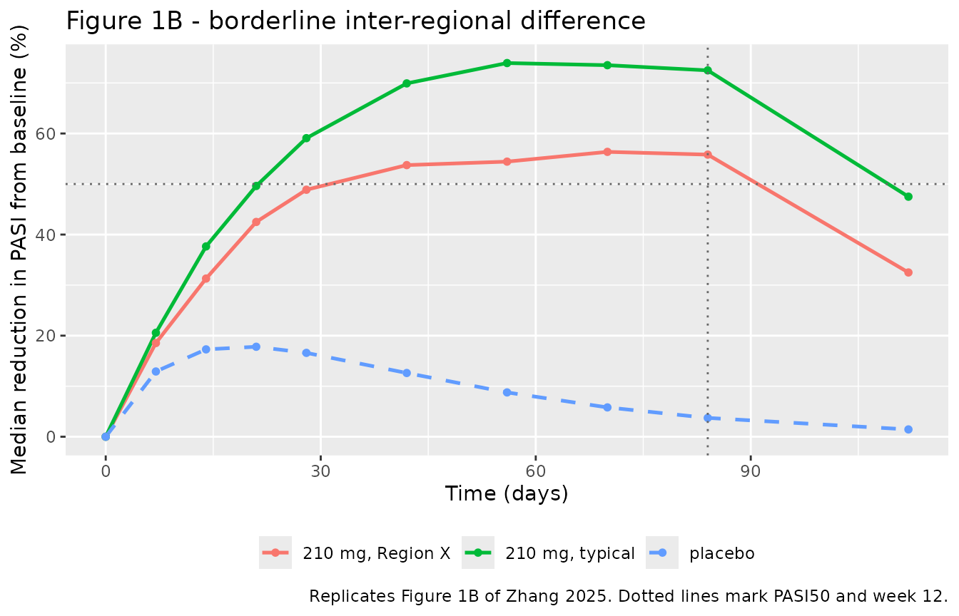
The placebo arm is shown once. Zhang 2025 draws two dashed placebo lines, one per region, but the regional covariate acts only on IC50, so with no drug on board the two placebo curves are identical by construction - which is why the figure’s dashed lines overlap.
feat <- resp |>
  dplyr::filter(treatment %in% c("210 mg, typical", "210 mg, Region X", "placebo")) |>
  dplyr::group_by(treatment) |>
  dplyr::summarise(
    `Peak reduction (%)`  = max(pct),
    `Day of peak`         = time[which.max(pct)],
    `Week 12 (%)`         = pct[time == 84],
    `Week 16 (%)`         = pct[time == 112],
    .groups = "drop"
  )
knitr::kable(feat, digits = 1,
caption = "Figure 1B features. Zhang 2025 shows the typical curve peaking near 69% around week 8 and recovering to about 48% by week 16; Region X reaching about 50% at week 12 and about 33% at week 16; and the placebo curve humping near 18% at weeks 2-3 before recovering.")| treatment | Peak reduction (%) | Day of peak | Week 12 (%) | Week 16 (%) |
|---|---|---|---|---|
| 210 mg, Region X | 55.3 | 56 | 49.3 | 31.2 |
| 210 mg, typical | 64.7 | 56 | 62.8 | 42.8 |
| placebo | 17.6 | 21 | 3.8 | 1.5 |
stopifnot(
  # Placebo response peaks early and then recovers - the counter-intuitive
  # shape produced by a placebo effect that is maximal at t = 0 and multiplies
  # the degradation rate. Zhang 2025 Figure 1B confirms it.
  feat$`Day of peak`[feat$treatment == "placebo"] >= 7,
  feat$`Day of peak`[feat$treatment == "placebo"] <= 28,
  feat$`Week 12 (%)`[feat$treatment == "placebo"] < 8,
  # Drug arms peak later and recover after the last dose at week 10.
  feat$`Day of peak`[feat$treatment == "210 mg, typical"] >= 42,
  feat$`Week 16 (%)`[feat$treatment == "210 mg, typical"] <
    feat$`Week 12 (%)`[feat$treatment == "210 mg, typical"]
)
Replicate Table 1: the regional effect ladder
Table 1 of Zhang 2025 maps the regional effect R_regionX
onto the median percentage PASI reduction at week 12 on 210 mg. It
publishes three anchors: 68.4% for typical patients
(R = 1.0), 50% at the borderline R = 2.6, and
a maximum inter-regional difference of 32.6 percentage points over the
scenario range R = 1.0 to 5.4, i.e. 35.8% at
R = 5.4.
Two simulated quantities are compared against those anchors, and they are not interchangeable:
- the typical-value trajectory
(
zeroRe(), all etas at zero), which is a deterministic ODE solve and therefore reproducible to solver precision across rxode2 versions; and - the population median over a 200-subject cohort, which is the same quantity the paper reports but carries Monte-Carlo noise.
With 136% CV on IC50 and a saturating response the two differ systematically - the median of the transform is not the transform of the median - so each is compared on its own terms, and the tight assertion is placed on the deterministic one.
r_ladder <- c(1.0, 1.8, 2.6, 5.4)

typ_w12 <- vapply(r_ladder, function(R) {
  m <- rxode2::ini(modz, e_region_china_ic50 = R)
  d <- rxode2::rxSolve(m, make_arm(1L, dose_q1w, 210, 1, "typ"),
                       omega = NA, useLinCmt = FALSE) |> as.data.frame()
  100 * (d$pasi[d$time == 0] - d$pasi[d$time == 84]) / d$pasi[d$time == 0]
}, numeric(1))
#> ℹ change initial estimate of `e_region_china_ic50` to `1`
#> ℹ change initial estimate of `e_region_china_ic50` to `1.8`
#> ℹ change initial estimate of `e_region_china_ic50` to `2.6`
#> ℹ change initial estimate of `e_region_china_ic50` to `5.4`
sim_w12 <- resp |>
  dplyr::filter(time == 84) |>
  dplyr::select(treatment, pop_median = pct)

tab1 <- tibble::tribble(
  ~treatment,                    ~R_regionX, ~published,
  "210 mg, typical",             1.0,        68.4,
  NA_character_,                 1.8,        NA_real_,
  "210 mg, Region X",            2.6,        50.0,
  "210 mg, Region X (R = 5.4)",  5.4,        35.8
) |>
  dplyr::mutate(typical = typ_w12) |>
  dplyr::left_join(sim_w12, by = "treatment") |>
  dplyr::mutate(typ_diff = typical - published,
                pop_diff = pop_median - published)

tab1 |>
  dplyr::select(R_regionX, published, typical, typ_diff, pop_median, pop_diff) |>
  dplyr::rename(
    "R_regionX"                          = R_regionX,
    "Published median reduction (%)"     = published,
    "Simulated typical value (%)"        = typical,
    "Typical - published (pp)"           = typ_diff,
    "Simulated population median (%)"    = pop_median,
    "Population - published (pp)"        = pop_diff
  ) |>
  knitr::kable(digits = 1,
caption = "Simulated vs published week-12 median PASI reduction on 210 mg (Zhang 2025 Table 1). R = 1.8 is the value Zhang 2025 Results names as the point above which the trial retains >50% power; the paper publishes no percentage reduction for it, and it was not one of the simulated cohorts.")| R_regionX | Published median reduction (%) | Simulated typical value (%) | Typical - published (pp) | Simulated population median (%) | Population - published (pp) |
|---|---|---|---|---|---|
| 1.0 | 68.4 | 73.5 | 5.1 | 62.8 | -5.6 |
| 1.8 | NA | 61.1 | NA | NA | NA |
| 2.6 | 50.0 | 52.4 | 2.4 | 49.3 | -0.7 |
| 5.4 | 35.8 | 35.6 | -0.2 | 34.5 | -1.3 |
anchored <- !is.na(tab1$published)

stopifnot(
  # --- Deterministic checks (no Monte-Carlo noise; solver-precision stable) ---
  # Table 1's ordering: a larger regional effect gives a smaller response.
  all(diff(tab1$typical) < 0),
  # Level agreement of the typical-value trajectory with the published medians.
  # The residual is the median-of-transform vs transform-of-median gap, which
  # for this model is at most about 5 percentage points.
  all(abs(tab1$typ_diff[anchored]) < 6),

  # --- Stochastic check (same quantity as the paper, but noisy) ---
  all(diff(tab1$pop_median[anchored]) < 0),
  # 10 pp, sized from the measured seed-to-seed spread of the 200-subject
  # median: across five seeds the typical arm ranged 64.9-71.2% and the
  # R = 2.6 arm 42.6-52.7%, against a published number computed from 21,000
  # subjects. Asserting tighter here would be asserting on Monte-Carlo noise
  # rather than on the model; the tight assertions are the deterministic ones
  # above.
  all(abs(tab1$pop_diff[anchored]) < 10)
)
Dose-regimen ranking
Methods 2.1 states that “among these dosing regimens, the 210 mg group will have the highest drug exposure” - the 280 mg arm is dosed only three times (weeks 0, 4 and 8) against seven doses for the weekly-then-biweekly arms. That is a falsifiable claim about the packaged model, and it is checked deterministically here. The same simulation exposes the model’s strong Michaelis-Menten nonlinearity: at 70 mg the absorbed input, 40 mg per dose over a 7- to 14-day interval, is at or below the 7.4 mg/day capacity of the saturable pathway, so almost no drug accumulates and the PASI response is close to placebo.
regimens <- tibble::tribble(
  ~treatment,     ~amt, ~days,
  "70 mg",        70,   dose_q1w,
  "140 mg",       140,  dose_q1w,
  "210 mg",       210,  dose_q1w,
  "280 mg Q4W",   280,  dose_q4w
)

ev_typ <- dplyr::bind_rows(lapply(seq_len(nrow(regimens)), function(i) {
  make_arm(1L, regimens$days[[i]], regimens$amt[i], 0, regimens$treatment[i],
           id_offset = i - 1L)
}))

sim_typ <- rxode2::rxSolve(modz, ev_typ, omega = NA,
                           keep = "treatment", useLinCmt = FALSE) |>
  as.data.frame()
#> Warning: multi-subject simulation without without 'omega'

dose_tab <- sim_typ |>
  dplyr::group_by(treatment) |>
  dplyr::summarise(
    `Peak Cc (ug/mL)`        = max(Cc),
    `Week 12 reduction (%)`  = 100 * (pasi[time == 0] - pasi[time == 84]) / pasi[time == 0],
    .groups = "drop"
  ) |>
  dplyr::arrange(match(treatment, regimens$treatment))

knitr::kable(dose_tab, digits = 2,
caption = "Typical-value exposure and week-12 response by regimen.")| treatment | Peak Cc (ug/mL) | Week 12 reduction (%) |
|---|---|---|
| 70 mg | 0.00 | 6.50 |
| 140 mg | 5.69 | 41.10 |
| 210 mg | 16.19 | 73.52 |
| 280 mg Q4W | 9.58 | 56.64 |
stopifnot(
  # The paper's stated ranking: 210 mg has the highest exposure of the four.
  dose_tab$`Peak Cc (ug/mL)`[dose_tab$treatment == "210 mg"] ==
    max(dose_tab$`Peak Cc (ug/mL)`),
  # Monotone dose-response within the common regimen.
  !is.unsorted(dose_tab$`Week 12 reduction (%)`[1:3]),
  # 280 mg Q4W sits below 210 mg on both exposure and response.
  dose_tab$`Week 12 reduction (%)`[dose_tab$treatment == "280 mg Q4W"] <
    dose_tab$`Week 12 reduction (%)`[dose_tab$treatment == "210 mg"]
)
sim_pd |>
  dplyr::filter(treatment != "placebo") |>
  dplyr::group_by(treatment, time) |>
  dplyr::summarise(Q05 = quantile(Cc, 0.05), Q50 = quantile(Cc, 0.50),
                   Q95 = quantile(Cc, 0.95), .groups = "drop") |>
  ggplot(aes(time, Q50, colour = treatment, fill = treatment)) +
  geom_ribbon(aes(ymin = Q05, ymax = Q95), alpha = 0.2, colour = NA) +
  geom_line(linewidth = 0.9) +
  labs(x = "Time (days)", y = "Cc (ug/mL)", colour = NULL, fill = NULL,
       title = "Simulated Drug A concentrations, 210 mg regimen",
       caption = "Median and 5th-95th percentiles. The regional covariate acts on IC50 only, so the two arms share a PK profile up to Monte-Carlo noise.") +
  theme(legend.position = "bottom")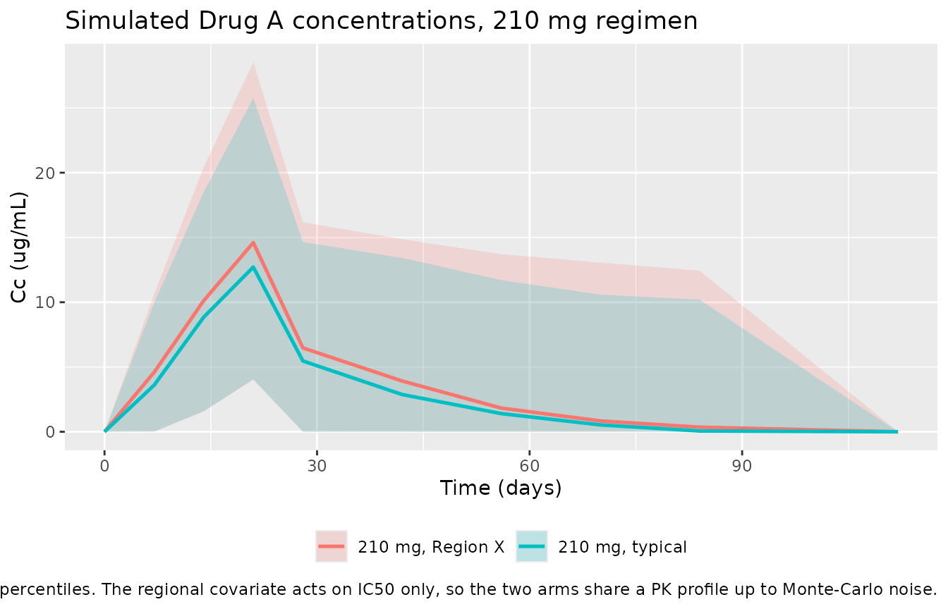
PKNCA validation
Zhang 2025 reports no NCA table, so there is nothing to compare against row-for-row. The NCA below instead characterises the packaged PK model and tests the one quantitative PK property the model asserts: elimination is partly saturable, so dose-normalised exposure must increase with dose.
A single-dose cohort is used, because NCA over the paper’s multiple-dose regimen would confound accumulation with saturation.
pk_times <- c(seq(0, 14, by = 1), seq(16, 84, by = 2), seq(88, 154, by = 6))
n_pk <- 100L

events_pk <- dplyr::bind_rows(lapply(seq_len(nrow(regimens)), function(i) {
  make_arm(n_pk, 0, regimens$amt[i], 0, regimens$treatment[i],
           id_offset = (i - 1L) * n_pk, obs_days = pk_times, obs_dvid = 1L)
}))
stopifnot(!anyDuplicated(events_pk[, c("id", "time", "evid")]))

rxode2::rxSetSeed(20250910)
sim_pk <- rxode2::rxSolve(mod, events_pk, omega = mod$omega,
                          keep = "treatment", useLinCmt = FALSE) |>
  as.data.frame()

# The stiff solver returns tiny negative values in the far tail once the
# saturable pathway has driven the concentration to essentially zero. Confirm
# they are numerical noise, then clamp so PKNCA does not take log() of a
# negative number.
stopifnot(min(sim_pk$Cc) > -1e-6)
sim_pk$Cc <- pmax(sim_pk$Cc, 0)
sim_nca <- sim_pk |>
  dplyr::filter(!is.na(Cc)) |>
  dplyr::select(id, time, Cc, treatment)

# Guarantee a time = 0 record per subject; for extravascular dosing Cc = 0 is
# the correct pre-dose value.
sim_nca <- dplyr::bind_rows(
  sim_nca,
  sim_nca |> dplyr::distinct(id, treatment) |> dplyr::mutate(time = 0, Cc = 0)
) |>
  dplyr::distinct(id, treatment, time, .keep_all = TRUE) |>
  dplyr::arrange(id, treatment, time)

conc_obj <- PKNCA::PKNCAconc(sim_nca, Cc ~ time | treatment + id)

dose_df <- events_pk |>
  dplyr::filter(evid == 1) |>
  dplyr::select(id, time, amt, treatment)
dose_obj <- PKNCA::PKNCAdose(dose_df, amt ~ time | treatment + id)

intervals <- data.frame(start = 0, end = max(pk_times),
                        cmax = TRUE, tmax = TRUE, auclast = TRUE)

nca_res <- PKNCA::pk.nca(PKNCA::PKNCAdata(conc_obj, dose_obj,
                                          intervals = intervals))
nca_tab <- as.data.frame(nca_res) |>
  dplyr::filter(PPTESTCD %in% c("cmax", "tmax", "auclast")) |>
  dplyr::group_by(treatment, PPTESTCD) |>
  dplyr::summarise(value = stats::median(PPORRES), .groups = "drop") |>
  tidyr::pivot_wider(names_from = PPTESTCD, values_from = value) |>
  dplyr::left_join(regimens |> dplyr::select(treatment, amt), by = "treatment") |>
  dplyr::mutate(dn_auclast = auclast / amt) |>
  dplyr::arrange(amt)

nca_tab |>
  # select() fixes the column ORDER so the positional `digits` vector below
  # lines up; rename() binds each header to its column BY NAME.
  dplyr::select(treatment, amt, cmax, tmax, auclast, dn_auclast) |>
  dplyr::rename(
    "Regimen"                         = treatment,
    "Dose (mg)"                       = amt,
    "Cmax (ug/mL)"                    = cmax,
    "Tmax (day)"                      = tmax,
    "AUClast (ug*day/mL)"             = auclast,
    "Dose-normalised AUClast (day/L)" = dn_auclast
  ) |>
  knitr::kable(digits = c(0, 0, 3, 1, 3, 4),
caption = "Single-dose NCA of the packaged model, median over 100 subjects per arm. No published NCA exists for this paper; the table characterises the model.")| Regimen | Dose (mg) | Cmax (ug/mL) | Tmax (day) | AUClast (ug*day/mL) | Dose-normalised AUClast (day/L) |
|---|---|---|---|---|---|
| 70 mg | 70 | 0.391 | 1 | 0.609 | 0.0087 |
| 140 mg | 140 | 2.688 | 2 | 13.185 | 0.0942 |
| 210 mg | 210 | 6.009 | 3 | 41.595 | 0.1981 |
| 280 mg Q4W | 280 | 10.502 | 4 | 102.642 | 0.3666 |
stopifnot(
  # Non-empty: guard against a filter chain that silently dropped every row.
  nrow(nca_tab) == nrow(regimens),
  # Cmax and AUC rise with dose.
  !is.unsorted(nca_tab$cmax),
  !is.unsorted(nca_tab$auclast),
  # The saturable pathway: dose-normalised exposure rises with dose. A purely
  # linear model would hold it constant.
  !is.unsorted(nca_tab$dn_auclast),
  # And the nonlinearity is large, not marginal.
  max(nca_tab$dn_auclast) / min(nca_tab$dn_auclast) > 5
)
Terminal half-life is deliberately not reported. With
Km = 0.01 ug/mL the saturable pathway is effectively
zero-order across the therapeutic range and becomes first-order only far
below it, so the apparent terminal slope is a function of concentration
rather than a system constant; a single half-life number for this model
would be misleading.
Assumptions and deviations
-
Simulation model, not a fit. Zhang 2025 does not
fit this model to Phase 2 data. Its parameters come from a Phase 1 D-E-R
model for Drug A “with minor adjustments” (Methods 2.2), and no
fitted-cohort demographics are published.
population$n_subjects = 175is the planned size of the simulated trial. -
The regional effect is a scenario value, not an
estimate.
R_regionXis fixed at 2.6, the borderline clinically relevant difference of Table 1 and the value the Data S4 generating script uses (COV_CN_VALUE_PD <- 2.6). The paper’s own re-estimation streams estimate it; Table 1 documents the full 1.0-to-5.4 range, and this vignette walks it. -
REGION_CHINAnames a region the article anonymises. The article says only “Region X”; the identification comes from the authors’ Data S4 code comments, as recorded in the covariate register entry and above. -
Erratum applied: Table S1’s PK additive residual
“SD (ug/mL) 0.09” is the
$SIGMAvariance; the packaged SD issqrt(0.09) = 0.3ug/mL. -
Control-stream unit comments overridden:
VMAX ug/dandka 1/hrin the Data S4 comments contradict Table S1 (mg/day, 1/day) and are dimensionally impossible; Table S1 is used. -
The
IF (TRT .EQ. 0) KSYN = KSYN0line is not reproduced. It exists in the control stream only because the placebo arm was dosed withAMT = 1e-10mg so that NONMEM would generate individual PK parameters for it. With a genuinely undosed placebo arm the effect-compartment concentration is identically zero andksynreduces toksyn0without a switch. -
Predictions, not observations. The figures and
tables use the model’s
Ccandpasipredictions (IPRED). Zhang 2025 simulated with residual error and summarised the resulting DV; the PASI residual error is small (6.36% proportional plus 1.145 PASI units additive) and symmetric, so the medians are materially unchanged. - Cohort size. 200 subjects per arm against the paper’s 21,000. The population-median column of the Table 1 comparison is therefore asserted only at 10 percentage points: with 136% CV on IC50 that median moves by several points from seed to seed, and it is not reproducible across rxode2 versions, which resample. The tight assertions are all on deterministic quantities - the two structural identities, the typical-value regional ladder (asserted at 6 pp against the published anchors and for exact monotonicity), the regimen ranking, and the dose-normalised AUC ordering.
- Age, weight, sex and race are not modelled. The published model has no covariates other than the regional indicator, so the virtual cohort carries none.