Tenofovir after tenofovir alafenamide in chronic kidney disease (Thoueille 2023)
Source:vignettes/articles/Thoueille_2023_tenofovir_ckd.Rmd
Thoueille_2023_tenofovir_ckd.RmdModel and source
This paper reports three independently fitted, independently
tabulated final models, so it contributes three model files to
nlmixr2lib and this single vignette ties them together.
| Model file | Paper’s model | Parameter table |
|---|---|---|
Thoueille_2023_tenofovir_reduced |
Tenofovir alone, creatinine clearance only (“reduced model”) | Table S2 |
Thoueille_2023_tenofovir_full |
Tenofovir alone, full covariate model (“final model”) | Table 2 |
Thoueille_2023_tenofovir_alafenamide |
Tenofovir alafenamide and tenofovir fitted simultaneously | Table S3 |
- Citation: Thoueille P, Alves Saldanha S, Desfontaine V, Kusejko K, Courlet P, Andre P, Cavassini M, Decosterd LA, Buclin T, Guidi M, and the Swiss HIV Cohort Study. Population pharmacokinetic modelling to characterize the effect of chronic kidney disease on tenofovir exposure after tenofovir alafenamide administration. J Antimicrob Chemother. 2023;78:1433-1443. doi:10.1093/jac/dkad103
- Article: https://doi.org/10.1093/jac/dkad103
- Supplement: available as Supplementary data at J Antimicrob Chemother Online
Tenofovir alafenamide is a prodrug of tenofovir that is taken up into cells and hydrolysed there, so the “absorption” step in these models represents the combined sequence of intestinal absorption, cellular uptake, intracellular conversion and release of tenofovir back into plasma. The authors show that this combined step is rate limiting, i.e. tenofovir displays flip-flop kinetics after tenofovir alafenamide dosing.
The reduced model is the one the authors recommend for routine therapeutic-drug-monitoring support, and every clinically relevant simulation in the paper (Figure 4, Figure 5, Table 3) is generated from it.
# Molar-mass constants. These are NOT from the paper -- the population analysis
# was run entirely in molar units (doses in nmol, concentrations in nmol/mL), so
# converting to the mass units used in the paper's own reported predictions
# (ng/mL, ng*h/mL) requires the molar masses. Values are the standard free-base
# molar masses (PubChem CID 9574768 for tenofovir alafenamide, CID 464205 for
# tenofovir).
MW_TAF <- 476.47 # g/mol, tenofovir alafenamide free base
MW_TFV <- 287.21 # g/mol, tenofovir free base

# Tenofovir alafenamide doses converted to nmol, exactly as the authors did.
dose_nmol <- function(mg) mg / MW_TAF * 1e6
DOSE_25 <- dose_nmol(25)
DOSE_10 <- dose_nmol(10)
c(`25 mg` = DOSE_25, `10 mg` = DOSE_10)
#>    25 mg    10 mg
#> 52469.20 20987.68
Population
The model-building dataset comprised 486 people living with HIV contributing 793 tenofovir concentrations, drawn from Swiss HIV Cohort Study project #815 and from the Lausanne routine therapeutic-drug-monitoring programme between January 2017 and January 2021 (Table 1). Median age was 51 years (range 19-79), median weight 74 kg (42-142), and 30% were female. Ethnicity was 71% White, 23% Black, 4% Hispanic American and 2% Asian. Renal function spanned a wide range, which is what makes the dataset informative about chronic kidney disease: median Cockcroft-Gault creatinine clearance 93 mL/min with a range of 33-203 mL/min, and median CKD-EPI eGFR 87 mL/min/1.73 m^2 (range 23-153).
Sampling was mostly sparse (one to two samples per subject), supplemented by four subjects with detailed 0-24 h profiles. Steady state was assumed for all individuals. Only 54 subjects contributed tenofovir alafenamide measurements (Table S1); because tenofovir alafenamide has a plasma half-life of roughly 0.5 h, only samples drawn within 6 h of dosing were assayed for it, yielding 100 samples of which 47 were below the limit of quantification. A further 83 subjects (84 observations) formed an external validation set that was not used for estimation; external validation of the tenofovir models gave a non-significant mean prediction error of 3.6% (95% CI 0.2-7.1%) with a precision of 17%.
The same information is available programmatically via each model’s
population metadata,
e.g. readModelDb("Thoueille_2023_tenofovir_reduced")()$population.
Source trace
Per-parameter origins are recorded as in-file comments next to each
ini() entry in the three files under
inst/modeldb/specificDrugs/. Collected here for review.
Reduced model (Thoueille_2023_tenofovir_reduced)
| Equation / parameter | Value | Source location |
|---|---|---|
lka (fixed) |
log(2) 1/h |
Table S2, k_a = “2 FIX”; rationale in Methods,
“Structural model” |
lcl |
log(43.2) L/h |
Table S2, CL_TFV
|
lvc |
log(2330) L |
Table S2, V_TFV
|
lfdepot (fixed) |
log(1) |
Table S2, F = “1 FIX” |
e_crcl_cl |
0.827 | Table S2, theta_CLCR; reference CLCR_ref =
100 mL/min (footnote) |
e_cobi_fdepot |
1.11 | Table S2, theta_Cobicistat
|
etalfdepot |
0.0493852 | Table S2, BSV on F = 22.5% CV;
omega^2 = log(1 + CV^2)
|
addSd |
0.0101 nmol/mL | Table S2, sigma_add
|
TVCL_TFV = CL_TFV * (1 + theta_CLCR * (CLCR - 100) / 100) |
n/a | Table S2, “Reduced model:” equation |
TVF = 1 + theta_Cobicistat |
n/a | Table S2, “Reduced model:” equation |
Full covariate model
(Thoueille_2023_tenofovir_full)
| Equation / parameter | Value | Source location |
|---|---|---|
lka (fixed) |
log(2) 1/h |
Table 2, k_a = “2 FIX” |
lcl |
log(42.2) L/h |
Table 2, CL_TFV
|
lvc |
log(2390) L |
Table 2, V_TFV
|
lfdepot (fixed) |
log(1) |
Table 2, F = “1 FIX” |
e_crcl_cl |
0.707 | Table 2, theta_CLCR; reference 100 mL/min |
e_age_cl |
-0.244 | Table 2, theta_Age; reference median 51 years |
e_race_black_hispanic_cl |
0.119 | Table 2, theta_Black or Hispano American
|
e_conmed_pgp_inh_cl |
-0.121 | Table 2, theta_Potent P-gp inhibitors
|
e_cobi_fdepot |
1.15 | Table 2, theta_Cobicistat
|
etalfdepot |
0.0435584 | Table 2, BSV on F = 21.1% CV |
addSd |
0.0099 nmol/mL | Table 2, sigma_add
|
Four-way multiplicative covariate product on
CL_TFV
|
n/a | Table 2, “Final model:” equation (identical form in Table S3) |
Joint tenofovir alafenamide + tenofovir model
(Thoueille_2023_tenofovir_alafenamide)
| Equation / parameter | Value | Source location |
|---|---|---|
lka (fixed) |
log(2) 1/h |
Table S3, k_12 = 2 (no RSE reported) |
lcl (tenofovir alafenamide) |
log(211) L/h |
Table S3, CL_TAF
|
lvc (tenofovir alafenamide) |
log(49.8) L |
Table S3, V_TAF
|
lcl_tfv |
log(42.2) L/h |
Table S3, CL_TFV
|
lvc_tfv |
log(2380) L |
Table S3, V_TFV
|
lfdepot (fixed) |
log(1) |
Table S3, F = “1 FIX” |
e_crcl_cl_tfv |
0.707 | Table S3, theta_CLCR
|
e_age_cl_tfv |
-0.250 | Table S3, theta_Age
|
e_race_black_hispanic_cl_tfv |
0.122 | Table S3, theta_Black or Hispano American
|
e_conmed_pgp_inh_cl_tfv |
-0.116 | Table S3, theta_Potent P-gp inhibitors
|
e_cobi_fdepot |
1.15 | Table S3, theta_Cobicistat
|
etalfdepot |
0.0439633 | Table S3, BSV on F = 21.2% CV |
etalcl |
0.6252023 | Table S3, BSV on CL_TAF = 93.2% CV |
propSd |
0.607 | Table S3, sigma_propTAF = 60.7 CV% |
addSd |
2.35e-3 nmol/mL | Table S3, sigma_addTAF = 2.35x10^-3 |
addSd_tfv |
9.92e-3 nmol/mL | Table S3, sigma_addTFV = 9.92x10^-3 |
Complete irreversible conversion, so
k23 = CL_TAF / V_TAF is the tenofovir input |
n/a | Methods, “Structural model”; Figure 2 upper panel |
Virtual cohort
Original observed data are not publicly available. The cohort below reproduces the paper’s own simulation design (Methods, “Model-based simulations”, and Supplementary “Simulations” item d): uniform creatinine-clearance distributions within each chronic-kidney-disease band, with the other covariates left at their reference values so that the renal-function effect is isolated.
set.seed(20230412) # advance-access publication date

N_PER_ARM <- 100L # 12 arms; well under the 200-per-arm cap

ckd_bands <- tibble::tribble(
  ~stage,        ~crcl_lo, ~crcl_hi,
  "Augmented",      150,      200,
  "Normal",          90,      149,
  "Stage 1",         60,       89,
  "Stage 2",         30,       59,
  "Stage 3",         15,       29,
  "Stage 4",          1,       15
)

regimens <- tibble::tribble(
  ~regimen,            ~amt,     ~cobi,
  "25 mg q.d.",        DOSE_25,  0L,
  "10 mg q.d. + COBI", DOSE_10,  1L
)

obs_grid <- seq(0, 24, by = 0.5)

# One arm = one CKD band x one regimen. `id_offset` keeps subject IDs disjoint
# across arms; duplicate IDs would be silently merged by rxSolve into a single
# subject receiving the summed dose.
make_arm <- function(stage, crcl_lo, crcl_hi, regimen, amt, cobi, id_offset) {
  subj <- tibble::tibble(
    id = id_offset + seq_len(N_PER_ARM),
    CRCL = runif(N_PER_ARM, crcl_lo, crcl_hi),
    CONMED_COBICISTAT = cobi,
    # Reference values for the covariates the paper held aside in this
    # simulation (Supplementary "Simulations" item d).
    AGE = 51,
    RACE_BLACK_HISPANIC = 0L,
    CONMED_PGP_INH = 0L,
    stage = stage,
    regimen = regimen,
    treatment = paste(stage, regimen, sep = " | ")
  )

  # Steady-state once-daily dosing into the depot, then a 0-24 h observation
  # grid on `central` (the ODE state -- never on the observable name `Cc`).
  doses <- subj |>
    dplyr::mutate(time = 0, amt = amt, evid = 1L, cmt = "depot",
                  ss = 1L, ii = 24)
  obs <- subj |>
    tidyr::crossing(time = obs_grid) |>
    dplyr::mutate(amt = NA_real_, evid = 0L, cmt = "central",
                  ss = NA_integer_, ii = NA_real_)

  dplyr::bind_rows(doses, obs) |>
    dplyr::arrange(id, time, dplyr::desc(evid))
}

arms <- tidyr::crossing(ckd_bands, regimens) |>
  dplyr::mutate(id_offset = (dplyr::row_number() - 1L) * N_PER_ARM)

events <- dplyr::bind_rows(lapply(seq_len(nrow(arms)), function(i) {
  a <- arms[i, ]
  make_arm(a$stage, a$crcl_lo, a$crcl_hi, a$regimen, a$amt, a$cobi, a$id_offset)
}))

stopifnot(!anyDuplicated(unique(events[, c("id", "time", "evid")])))
dplyr::n_distinct(events$id)
#> [1] 1200
Simulation
mod_reduced <- readModelDb("Thoueille_2023_tenofovir_reduced")

sim <- rxode2::rxSolve(
  mod_reduced,
  events = events,
  keep = c("stage", "regimen", "treatment", "CRCL"),
  # steady-state searches for long-half-life subjects exceed the default step budget
  maxsteps = 1e6
) |>
  as.data.frame() |>
  # Model concentrations are nmol/mL; the paper reports ng/mL.
  dplyr::mutate(Cc_ngml = Cc * MW_TFV)
#> ℹ parameter labels from comments will be replaced by 'label()'

dplyr::glimpse(dplyr::select(sim, id, time, Cc, Cc_ngml, stage, regimen))
#> Rows: 58,800
#> Columns: 6
#> $ id      <int> 1, 1, 1, 1, 1, 1, 1, 1, 1, 1, 1, 1, 1, 1, 1, 1, 1, 1, 1, 1, 1,…
#> $ time    <dbl> 0.0, 0.5, 1.0, 1.5, 2.0, 2.5, 3.0, 3.5, 4.0, 4.5, 5.0, 5.5, 6.…
#> $ Cc      <dbl> 0.01630424, 0.02662624, 0.03011737, 0.03110011, 0.03116452, 0.…
#> $ Cc_ngml <dbl> 4.682742, 7.647322, 8.650011, 8.932262, 8.950763, 8.873503, 8.…
#> $ stage   <chr> "Augmented", "Augmented", "Augmented", "Augmented", "Augmented…
#> $ regimen <chr> "10 mg q.d. + COBI", "10 mg q.d. + COBI", "10 mg q.d. + COBI",…
Replicate published figures
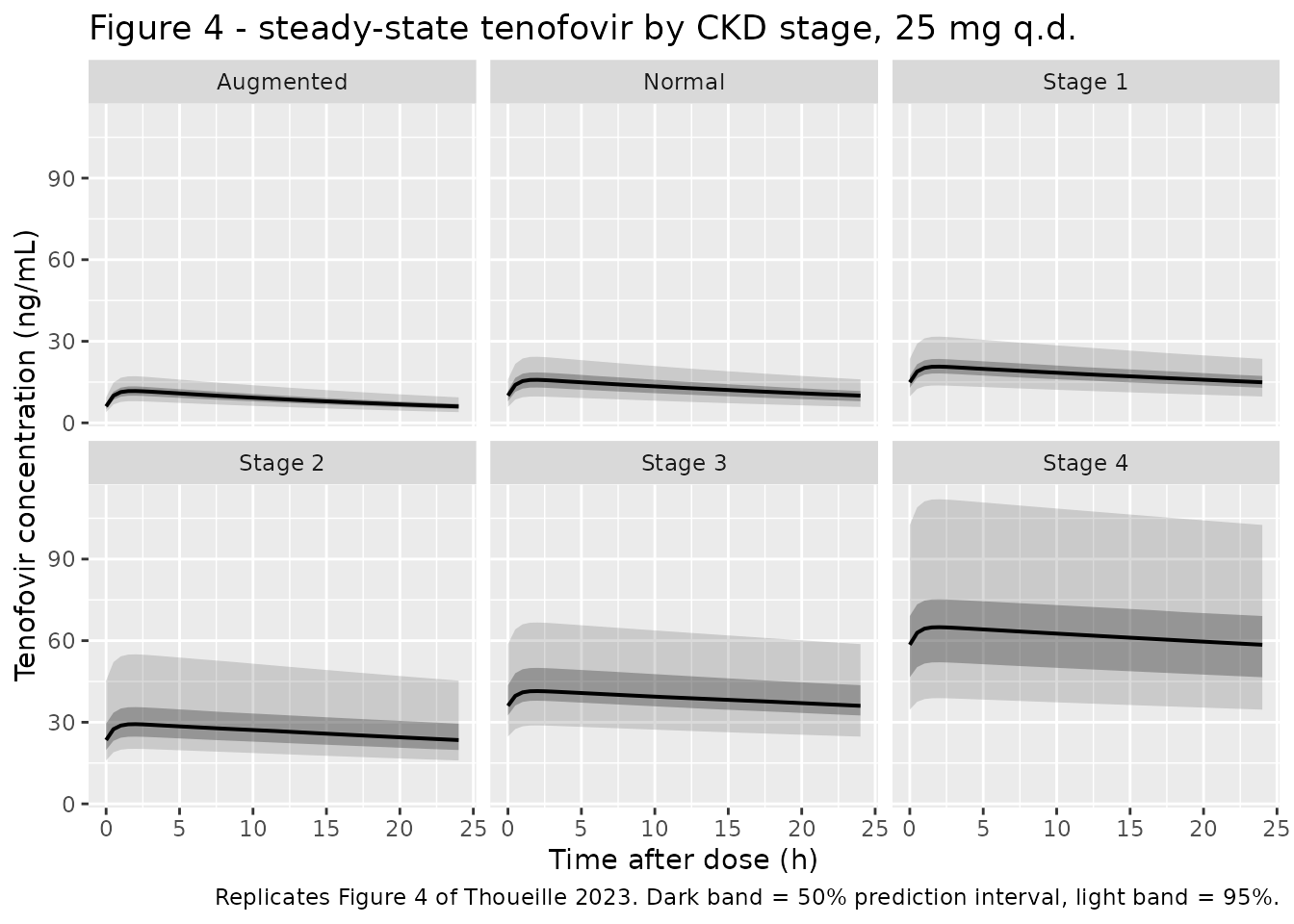
# Replicates Figure 4 of Thoueille 2023: simulated steady-state tenofovir
# profiles after 25 mg tenofovir alafenamide, by CKD stage.
sim |>
  dplyr::filter(regimen == "25 mg q.d.") |>
  dplyr::mutate(stage = factor(stage, levels = ckd_bands$stage)) |>
  dplyr::group_by(stage, time) |>
  dplyr::summarise(
    Q025 = quantile(Cc_ngml, 0.025),
    Q250 = quantile(Cc_ngml, 0.250),
    Q500 = quantile(Cc_ngml, 0.500),
    Q750 = quantile(Cc_ngml, 0.750),
    Q975 = quantile(Cc_ngml, 0.975),
    .groups = "drop"
  ) |>
  ggplot(aes(time, Q500)) +
  geom_ribbon(aes(ymin = Q025, ymax = Q975), alpha = 0.18) +
  geom_ribbon(aes(ymin = Q250, ymax = Q750), alpha = 0.35) +
  geom_line(linewidth = 0.7) +
  facet_wrap(~stage) +
  labs(
    x = "Time after dose (h)", y = "Tenofovir concentration (ng/mL)",
    title = "Figure 4 - steady-state tenofovir by CKD stage, 25 mg q.d.",
    caption = paste(
      "Replicates Figure 4 of Thoueille 2023. Dark band = 50% prediction",
      "interval, light band = 95%."
    )
  )
# Replicates Figure 5 of Thoueille 2023: the proposed dosage-interval
# adjustment for stage 3 and stage 4 CKD (one dose every 2 and 3 days
# respectively) compared with unadjusted once-daily dosing.
adjust_arms <- tibble::tribble(
  ~stage,     ~crcl_lo, ~crcl_hi, ~ii_adj,
  "Stage 3",       15,       29,       48,
  "Stage 4",        1,       15,       72
)

make_adjusted <- function(stage, crcl_lo, crcl_hi, ii_adj, id_offset) {
  subj <- tibble::tibble(
    id = id_offset + seq_len(N_PER_ARM),
    CRCL = runif(N_PER_ARM, crcl_lo, crcl_hi),
    CONMED_COBICISTAT = 0L, AGE = 51,
    RACE_BLACK_HISPANIC = 0L, CONMED_PGP_INH = 0L,
    stage = stage,
    schedule = paste0("every ", ii_adj / 24, " days")
  )
  doses <- subj |>
    dplyr::mutate(time = 0, amt = DOSE_25, evid = 1L, cmt = "depot",
                  ss = 1L, ii = ii_adj)
  obs <- subj |>
    tidyr::crossing(time = seq(0, ii_adj, by = 1)) |>
    dplyr::mutate(amt = NA_real_, evid = 0L, cmt = "central",
                  ss = NA_integer_, ii = NA_real_)
  dplyr::bind_rows(doses, obs) |>
    dplyr::arrange(id, time, dplyr::desc(evid))
}

adjust_arms2 <- adjust_arms |> dplyr::mutate(id_offset = c(20000L, 21000L))
events_adj <- dplyr::bind_rows(lapply(seq_len(nrow(adjust_arms2)), function(i) {
  a <- adjust_arms2[i, ]
  make_adjusted(a$stage, a$crcl_lo, a$crcl_hi, a$ii_adj, a$id_offset)
}))

sim_adj <- rxode2::rxSolve(
  mod_reduced, events = events_adj,
  keep = c("stage", "schedule", "CRCL"),
  # steady-state searches for long-half-life subjects exceed the default step budget
  maxsteps = 1e6
) |>
  as.data.frame() |>
  dplyr::mutate(Cc_ngml = Cc * MW_TFV)

dplyr::bind_rows(
  sim |>
    dplyr::filter(regimen == "25 mg q.d.", stage %in% adjust_arms$stage) |>
    dplyr::mutate(schedule = "every 1 day (unadjusted)"),
  sim_adj
) |>
  dplyr::group_by(stage, schedule, time) |>
  dplyr::summarise(
    Q025 = quantile(Cc_ngml, 0.025),
    Q500 = quantile(Cc_ngml, 0.500),
    Q975 = quantile(Cc_ngml, 0.975),
    .groups = "drop"
  ) |>
  ggplot(aes(time, Q500, fill = schedule, colour = schedule)) +
  geom_ribbon(aes(ymin = Q025, ymax = Q975), alpha = 0.25, colour = NA) +
  geom_line(linewidth = 0.7) +
  facet_wrap(~stage, scales = "free_x") +
  labs(
    x = "Time after dose (h)", y = "Tenofovir concentration (ng/mL)",
    title = "Figure 5 - proposed dosage-interval adjustment in stage 3 / 4 CKD",
    caption = "Replicates Figure 5 of Thoueille 2023."
  ) +
  theme(legend.position = "bottom")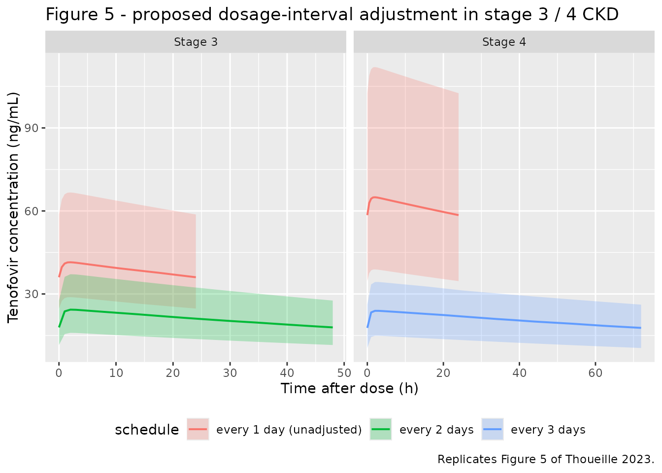
Covariate effects of the full model
The paper quotes two typical-value clearances from the full model as
a sanity check on the covariate coefficients: 18 L/h at a creatinine
clearance of 20 mL/min (“57% lower” than normal), and 36 L/h at age 80
versus 42 L/h at the median age of 51. Reading cl straight
out of the solved full model confirms the encoded covariate algebra.
mod_full <- readModelDb("Thoueille_2023_tenofovir_full") |> rxode2::zeroRe()
#> ℹ parameter labels from comments will be replaced by 'label()'

probe <- tibble::tribble(
  ~label,                       ~CRCL, ~AGE,
  "CLCR 100 mL/min, age 51",      100,   51,
  "CLCR 20 mL/min (stage 3)",      20,   51,
  "Age 80 y, CLCR 100 mL/min",    100,   80
) |>
  dplyr::mutate(
    id = dplyr::row_number(),
    RACE_BLACK_HISPANIC = 0L, CONMED_PGP_INH = 0L, CONMED_COBICISTAT = 0L
  )

probe_events <- dplyr::bind_rows(
  probe |> dplyr::mutate(time = 0, amt = DOSE_25, evid = 1L, cmt = "depot"),
  probe |> dplyr::mutate(time = 24, amt = NA_real_, evid = 0L, cmt = "central")
) |>
  dplyr::arrange(id, time, dplyr::desc(evid))

rxode2::rxSolve(mod_full, events = probe_events, keep = c("label")) |>
  as.data.frame() |>
  dplyr::filter(!is.na(cl)) |>
  dplyr::group_by(label) |>
  dplyr::summarise(`CL/F (L/h)` = round(mean(cl), 1), .groups = "drop") |>
  dplyr::mutate(`Paper (L/h)` = c(42, 18, 36)[match(
    label, c("CLCR 100 mL/min, age 51", "CLCR 20 mL/min (stage 3)",
             "Age 80 y, CLCR 100 mL/min"))]) |>
  dplyr::rename("Scenario" = label) |>
  knitr::kable(caption = paste(
    "Full-model typical clearance versus the values quoted in Thoueille 2023",
    "Results ('Structural, statistical and covariate models')."
  ))
#> ℹ omega/sigma items treated as zero: 'etalfdepot'
#> Warning: multi-subject simulation without without 'omega'| Scenario | CL/F (L/h) | Paper (L/h) |
|---|---|---|
| Age 80 y, CLCR 100 mL/min | 36.3 | 36 |
| CLCR 100 mL/min, age 51 | 42.2 | 42 |
| CLCR 20 mL/min (stage 3) | 18.3 | 18 |
Joint model: flip-flop kinetics and agreement with the tenofovir-alone fit
The joint model lets tenofovir alafenamide be observed directly. Two
published claims are checked here. First, flip-flop kinetics: the
absorption rate constant k12 (2 1/h, fixed) must be smaller
than the conversion rate constant k23 = CL_TAF / V_TAF.
Second, the paper states the joint model “provided exactly the same
description and parameter values for tenofovir as the model developed
from the tenofovir data alone”, so the two tenofovir profiles should be
close. They are not bit-identical: at the reference covariates both
models share CL_TFV = 42.2 L/h and differ only in
V_TFV (2380 versus 2390 L), but the joint model routes
tenofovir through an extra prodrug compartment, so its tenofovir input
is slightly smoothed relative to the tenofovir-alone model’s direct
first-order absorption. The residual disagreement is confined to the
absorption phase and is quantified below.
mod_joint <- readModelDb("Thoueille_2023_tenofovir_alafenamide") |> rxode2::zeroRe()
#> ℹ parameter labels from comments will be replaced by 'label()'

k12 <- 2
k23 <- 211 / 49.8 # Table S3: CL_TAF / V_TAF
cat(sprintf("k12 = %.2f 1/h; k23 = %.2f 1/h; flip-flop (k12 < k23): %s\n",
            k12, k23, k12 < k23))
#> k12 = 2.00 1/h; k23 = 4.24 1/h; flip-flop (k12 < k23): TRUE

joint_events <- {
  subj <- tibble::tibble(
    id = 1L, CRCL = 100, AGE = 51,
    RACE_BLACK_HISPANIC = 0L, CONMED_PGP_INH = 0L, CONMED_COBICISTAT = 0L
  )
  dplyr::bind_rows(
    subj |> dplyr::mutate(time = 0, amt = DOSE_25, evid = 1L, cmt = "depot",
                          ss = 1L, ii = 24, dvid = 1L),
    subj |> tidyr::crossing(time = seq(0, 24, by = 0.25)) |>
      dplyr::mutate(amt = NA_real_, evid = 0L, cmt = "central",
                    ss = NA_integer_, ii = NA_real_, dvid = 1L)
  ) |>
    dplyr::arrange(id, time, dplyr::desc(evid))
}

# This model declares two endpoints (`Cc` and `Cc_tfv`) and BOTH are algebraic
# observables rather than ODE states, so rxode2's dvid->cmt map has no
# "endpoint that is also a state" to point `cmt` at. Observation rows therefore
# carry the ODE state name plus an explicit `dvid`; `cmt = "central"` alone
# fails with "'dvid'->'cmt' ... on a undefined compartment". `dvid` is set on
# the dose rows too so the column is not NA-typed. rxode2 still returns both
# observables as columns on every observation row.
# steady-state searches for long-half-life subjects exceed the default step budget
sim_joint <- rxode2::rxSolve(mod_joint, events = joint_events,
                             maxsteps = 1e6) |>
  as.data.frame()
#> ℹ omega/sigma items treated as zero: 'etalfdepot', 'etalcl'

# Same scenario through the tenofovir-alone full model, which has a single
# endpoint and so needs no dvid column.
alone_events <- joint_events |> dplyr::select(-dvid)
# steady-state searches for long-half-life subjects exceed the default step budget
sim_alone <- rxode2::rxSolve(mod_full, events = alone_events,
                             maxsteps = 1e6) |>
  as.data.frame()
#> ℹ omega/sigma items treated as zero: 'etalfdepot'

dplyr::bind_rows(
  tibble::tibble(time = sim_joint$time, conc = sim_joint$Cc * MW_TAF,
                 analyte = "Tenofovir alafenamide (joint model)"),
  tibble::tibble(time = sim_joint$time, conc = sim_joint$Cc_tfv * MW_TFV,
                 analyte = "Tenofovir (joint model)"),
  tibble::tibble(time = sim_alone$time, conc = sim_alone$Cc * MW_TFV,
                 analyte = "Tenofovir (tenofovir-alone full model)")
) |>
  ggplot(aes(time, conc, colour = analyte, linetype = analyte)) +
  geom_line(linewidth = 0.7) +
  scale_y_log10() +
  labs(
    x = "Time after dose (h)", y = "Concentration (ng/mL)",
    title = "Joint tenofovir alafenamide / tenofovir model at steady state",
    caption = paste(
      "Tenofovir alafenamide falls fast (half-life ~0.5 h) while tenofovir",
      "accumulates - the flip-flop behaviour described in Thoueille 2023",
      "Results. The two tenofovir curves are nearly indistinguishable on this",
      "scale, consistent with the paper's claim that the joint fit and the",
      "tenofovir-alone fit give the same tenofovir description."
    )
  ) +
  theme(legend.position = "bottom", legend.direction = "vertical")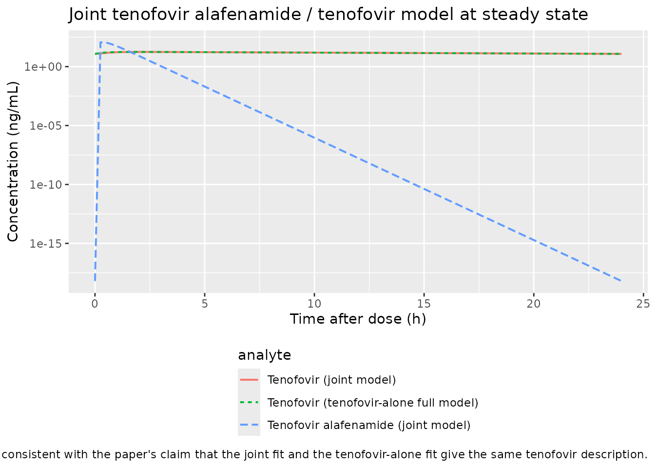
# Quantify the superposition claim rather than relying on the eye.
agree <- dplyr::inner_join(
  sim_joint |> dplyr::select(time, joint = Cc_tfv),
  sim_alone |> dplyr::select(time, alone = Cc),
  by = "time"
) |>
  dplyr::filter(time > 0) |>
  dplyr::mutate(pct_diff = 100 * (joint - alone) / alone)

sprintf(
  "Tenofovir profile agreement, joint vs tenofovir-alone: max |difference| = %.2f%% over 0-24 h",
  max(abs(agree$pct_diff))
)
#> [1] "Tenofovir profile agreement, joint vs tenofovir-alone: max |difference| = 9.79% over 0-24 h"
PKNCA validation
The paper’s Table 3 reports model-predicted steady-state
AUC0-24 and trough concentration (Cmin) for
each CKD stage under both regimens, derived from the reduced model. NCA
on the simulated profiles reproduces those metrics.
sim_nca <- sim |>
  dplyr::filter(!is.na(Cc_ngml)) |>
  dplyr::transmute(id, time, Cc = Cc_ngml, treatment) |>
  dplyr::arrange(id, treatment, time)

# PKNCA anchors AUC0-24 at the interval start, so every subject needs a
# time = 0 record. The observation grid begins at 0 and `ss = 1` makes that
# record the steady-state trough (NOT zero -- this is a steady-state interval,
# so back-filling a pre-dose zero would corrupt both AUC0-24 and Cmin).
# Assert the row is present rather than fabricating one.
stopifnot(all(
  sim_nca |>
    dplyr::group_by(id) |>
    dplyr::summarise(has_t0 = any(dplyr::near(time, 0)), .groups = "drop") |>
    dplyr::pull(has_t0)
))

conc_obj <- PKNCA::PKNCAconc(
  sim_nca, Cc ~ time | treatment + id,
  concu = "ng/mL", timeu = "h"
)

dose_df <- events |>
  dplyr::filter(evid == 1) |>
  dplyr::select(id, time, amt, treatment)

dose_obj <- PKNCA::PKNCAdose(dose_df, amt ~ time | treatment + id, doseu = "nmol")

# At steady state with once-daily dosing the interval minimum is the trough, so
# `cmin` is the paper's Cmin; `auclast` over 0-24 h is its AUC0-24.
intervals <- data.frame(
  start = 0, end = 24,
  auclast = TRUE, cmax = TRUE, tmax = TRUE, cmin = TRUE
)

nca_res <- PKNCA::pk.nca(PKNCA::PKNCAdata(conc_obj, dose_obj, intervals = intervals))
Comparison against published NCA
# Thoueille 2023 Table 3, transcribed. AUC0-24 in ng*h/mL, Cmin in ng/mL.
published <- tibble::tribble(
  ~treatment,                       ~auclast, ~cmin,
  "Augmented | 25 mg q.d.",              218,   6.4,
  "Normal | 25 mg q.d.",                 298,   9.7,
  "Stage 1 | 25 mg q.d.",                444,  15.7,
  "Stage 2 | 25 mg q.d.",                660,  24.5,
  "Stage 3 | 25 mg q.d.",               1000,  38.9,
  "Stage 4 | 25 mg q.d.",               1610,  64.1,
  "Augmented | 10 mg q.d. + COBI",       183,   5.3,
  "Normal | 10 mg q.d. + COBI",          257,   8.3,
  "Stage 1 | 10 mg q.d. + COBI",         374,  13.2,
  "Stage 2 | 10 mg q.d. + COBI",         555,  20.7,
  "Stage 3 | 10 mg q.d. + COBI",         854,  33.1,
  "Stage 4 | 10 mg q.d. + COBI",        1325,  52.7
)

cmp <- nlmixr2lib::ncaComparisonTable(
  simulated = nca_res,
  reference = published,
  by = "treatment",
  units = c(auclast = "ng*h/mL", cmin = "ng/mL"),
  tolerance_pct = 20
)

knitr::kable(
  cmp,
  caption = paste(
    "Simulated versus published (Thoueille 2023 Table 3) steady-state",
    "tenofovir exposure by CKD stage and regimen.",
    "* differs from reference by >20%."
  ),
  align = c("l", "l", "r", "r", "r")
)| NCA parameter | treatment | Reference | Simulated | % diff |
|---|---|---|---|---|
| Cmin (ng/mL) | Augmented | 25 mg q.d. | 6.4 | 6.05 | -5.5% |
| Cmin (ng/mL) | Normal | 25 mg q.d. | 9.7 | 10 | +3.3% |
| Cmin (ng/mL) | Stage 1 | 25 mg q.d. | 15.7 | 14.9 | -5.0% |
| Cmin (ng/mL) | Stage 2 | 25 mg q.d. | 24.5 | 23.4 | -4.3% |
| Cmin (ng/mL) | Stage 3 | 25 mg q.d. | 38.9 | 36 | -7.3% |
| Cmin (ng/mL) | Stage 4 | 25 mg q.d. | 64.1 | 58.5 | -8.7% |
| Cmin (ng/mL) | Augmented | 10 mg q.d. + COBI | 5.3 | 5.33 | +0.6% |
| Cmin (ng/mL) | Normal | 10 mg q.d. + COBI | 8.3 | 8.25 | -0.6% |
| Cmin (ng/mL) | Stage 1 | 10 mg q.d. + COBI | 13.2 | 13 | -1.3% |
| Cmin (ng/mL) | Stage 2 | 10 mg q.d. + COBI | 20.7 | 20.8 | +0.5% |
| Cmin (ng/mL) | Stage 3 | 10 mg q.d. + COBI | 33.1 | 32.2 | -2.6% |
| Cmin (ng/mL) | Stage 4 | 10 mg q.d. + COBI | 52.7 | 50.3 | -4.5% |
| AUClast (ng*h/mL) | Augmented | 25 mg q.d. | 218 | 210 | -3.8% |
| AUClast (ng*h/mL) | Normal | 25 mg q.d. | 298 | 308 | +3.4% |
| AUClast (ng*h/mL) | Stage 1 | 25 mg q.d. | 444 | 428 | -3.6% |
| AUClast (ng*h/mL) | Stage 2 | 25 mg q.d. | 660 | 637 | -3.5% |
| AUClast (ng*h/mL) | Stage 3 | 25 mg q.d. | 1000 | 932 | -6.8% |
| AUClast (ng*h/mL) | Stage 4 | 25 mg q.d. | 1610 | 1480 | -7.8% |
| AUClast (ng*h/mL) | Augmented | 10 mg q.d. + COBI | 183 | 180 | -1.7% |
| AUClast (ng*h/mL) | Normal | 10 mg q.d. + COBI | 257 | 250 | -2.6% |
| AUClast (ng*h/mL) | Stage 1 | 10 mg q.d. + COBI | 374 | 372 | -0.6% |
| AUClast (ng*h/mL) | Stage 2 | 10 mg q.d. + COBI | 555 | 560 | +0.9% |
| AUClast (ng*h/mL) | Stage 3 | 10 mg q.d. + COBI | 854 | 836 | -2.1% |
| AUClast (ng*h/mL) | Stage 4 | 10 mg q.d. + COBI | 1320 | 1280 | -3.8% |
# The paper's headline result: percentage change in median Cmin relative to
# normal renal function (Results, "Simulations": 59%, 143%, 294% and 515%
# increases for stages 1-4, and a 36% decrease with augmented function).
med_cmin <- sim |>
  dplyr::filter(regimen == "25 mg q.d.", dplyr::near(time, 24)) |>
  dplyr::group_by(stage) |>
  dplyr::summarise(cmin = median(Cc_ngml), .groups = "drop")

ref_cmin <- med_cmin$cmin[med_cmin$stage == "Normal"]

med_cmin |>
  dplyr::mutate(
    `Simulated change vs normal (%)` = round(100 * (cmin / ref_cmin - 1)),
    `Paper change vs normal (%)` = c(-36, NA, 59, 143, 294, 515)[
      match(stage, c("Augmented", "Normal", "Stage 1", "Stage 2",
                     "Stage 3", "Stage 4"))],
    `Median Cmin (ng/mL)` = round(cmin, 1)
  ) |>
  dplyr::select(stage, `Median Cmin (ng/mL)`,
                `Simulated change vs normal (%)`,
                `Paper change vs normal (%)`) |>
  dplyr::rename("CKD stage" = stage) |>
  knitr::kable(caption = paste(
    "Median steady-state trough tenofovir by renal function, 25 mg q.d.,",
    "against the percentage changes reported in Thoueille 2023 Results."
))| CKD stage | Median Cmin (ng/mL) | Simulated change vs normal (%) | Paper change vs normal (%) |
|---|---|---|---|
| Augmented | 6.1 | -40 | -36 |
| Normal | 10.0 | 0 | NA |
| Stage 1 | 14.9 | 49 | 59 |
| Stage 2 | 23.4 | 134 | 143 |
| Stage 3 | 36.0 | 260 | 294 |
| Stage 4 | 58.5 | 484 | 515 |
Assumptions and deviations
-
Stage 4 creatinine-clearance range. The paper
defines stage 4 only as
CLCR < 15 mL/minwith no lower bound (Methods, “Model-based simulations”). A uniform distribution over 1-15 mL/min is used here. The paper’s own median stage-4 predictions correspond to a median creatinine clearance nearer 5 mL/min, so the simulated stage-4 exposures here run modestly below the published values; this is a consequence of the unstated lower bound, not of the model parameters. All other bands use the paper’s stated ranges verbatim. -
Augmented renal function. Methods states “augmented
kidney function: 200-150 mL/min” while the abstract and Figure S6
caption describe it as
CLCR > 149 mL/min. The Methods range (150-200) is used, since that is what the simulation section specifies. -
Molar-mass constants are not from the paper. The
population analysis is entirely in molar units, so
MW_TAF = 476.47 g/molandMW_TFV = 287.21 g/mol(standard free-base molar masses, PubChem) are needed to express results in the ng/mL and ng*h/mL units the paper reports. They are unit conversions, not model parameters, and are therefore defined in this vignette rather than inini(). -
Concentration scale in
model(). Amounts are in nmol and volumes in L, soamount / volumeis nmol/L. Each model divides by a further 1000 so thatCcis on the nmol/mL scale the authors used for the concentrations and for the residual-error estimates; this keeps everyini()value byte-identical to the published tables instead of silently rescalingsigma_add. -
Between-subject variability expressed as CV%. The
papers’s tables report BSV as a percentage and the Methods state
parameters were log-normally distributed, so variances are entered as
omega^2 = log(1 + CV^2). -
Steady state assumed. The authors assumed steady
state for every individual, so the simulations use
ss = 1with the relevant dosing interval rather than dosing forward from time zero. - Covariates held at reference values. Figure 4 and Table 3 come from the reduced model, which contains only creatinine clearance and cobicistat, so age, ethnicity and P-gp-inhibitor comedication do not enter those simulations. For the full-model probe they are set to the reference categories (age 51 years, not Black or Hispanic American, no potent P-gp inhibitor) so the reported coefficient is isolated.
-
Cobicistat is confounded with dose level. Every
cobicistat-treated subject received 10 mg tenofovir alafenamide and
every other subject 25 mg, because cobicistat was forced into the model
specifically to absorb the dose difference into relative
bioavailability.
e_cobi_fdepottherefore represents a combined dose-normalisation and boosting effect, not a pure drug-drug interaction; it cannot be reused as a standalone cobicistat interaction term. -
Only the potent P-gp-inhibitor tier is encoded. The
paper screened potent inhibitors, moderate inhibitors and inducers as
three separate strata and retained only the potent one.
CONMED_PGP_INHtherefore carries the potent tier alone in these models; moderate inhibitors and inducers are recorded incovariatesDataExcluded. -
“Exactly the same description” is approximate, not
literal. The paper states the joint model gives “exactly the
same description and parameter values for tenofovir” as the
tenofovir-alone model. The parameter values do match at the reference
covariates (
CL_TFV42.2 L/h in both;V_TFV2380 versus 2390 L), but the two structures are not identical: the joint model passes the dose through a tenofovir alafenamide compartment before tenofovir, whereas the tenofovir-alone model absorbs directly into tenofovir. Simulated tenofovir profiles therefore differ by up to ~10% during the absorption phase and are effectively identical thereafter. Neither model was altered to close that gap. - Figure 3 (the visual predictive checks) and the diagnostic plots are not reproduced, since they require the observed concentrations, which are not publicly available.
- The Figure S5 age + creatinine-clearance variant is not packaged. It has published equations but no parameter table of its own; it reuses the full model’s coefficients and is a simulation aid rather than a separately fitted model.
-
The base model is not packaged either. The
V_TFVof 2660 L /CL_TFVof 39.9 L/h base-model values quoted in Results (and the derived half-life of 46 h andTmaxof 2.4 h) precede covariate inclusion and are superseded by the three final models. -
New canonical names registered with this extraction
(ratified by the maintainers on 2026-07-29): the metabolite suffix
tfv, the composite race columnRACE_BLACK_HISPANIC, the class-level comedication columnCONMED_PGP_INH, andCONMED_COBICISTAT. In the joint model tenofovir alafenamide is the dosed parent and so keeps the canonicalcentral/Ccnames, with tenofovir carrying the_tfvsuffix; in the two tenofovir-alone models tenofovir itself iscentral/Cc. That difference follows the register’s “the parent always wins canonical naming” rule.