Cabotegravir thigh injection (Han 2024)
Source:vignettes/articles/Han_2024_cabotegravir.Rmd
Han_2024_cabotegravir.RmdModel and source
- Citation: Han K, D’Amico RD, Spreen WR, Ford SL. Population pharmacokinetics of cabotegravir following intramuscular thigh injections in adults with and without HIV. Antimicrob Agents Chemother. 2024;68(12):e00880-24. doi:10.1128/aac.00880-24. Fixed parameters from: Han K, Baker M, Lovern M, et al. Br J Clin Pharmacol. 2022;88(10):4607-4622. doi:10.1111/bcp.15439
- Description: Two-compartment population PK model for cabotegravir after oral tablets and long-acting (LA) intramuscular injections into either the gluteal or the lateral thigh (vastus lateralis) muscle, in adults with and without HIV-1 (Han 2024, phase 1 study 208832 and the ATLAS-2M thigh PK substudy). Three parallel first-order depots (oral, IM gluteal, IM thigh) feed one central compartment, so a gluteal depot and a thigh depot can absorb at the same time when the injection site is switched. Only the thigh absorption rate constant and the thigh bioavailability were estimated; every other parameter is fixed to the Han 2022 oral + gluteal model. The typical thigh absorption rate constant is the typical gluteal value plus 0.0002527 1/h, so it inherits the gluteal effects of sex, BMI, split injection and needle length; thigh bioavailability is 89.9% of gluteal.
- Article: Antimicrob Agents Chemother 2024;68(12):e00880-24 (open access, PMC11619381)
Long-acting (LA) cabotegravir is approved as an intramuscular (IM)
gluteal injection. Han 2024 asked whether the lateral thigh (vastus
lateralis) is a workable alternative site. The authors took the Han 2022
oral + gluteal population PK model (packaged as
Han_2022_cabotegravir), added a thigh injection depot, and
fitted only the thigh absorption rate constant and the thigh
bioavailability. Every other parameter stayed fixed at its Han 2022
value.
The model has three depots, all emptying into one two-compartment disposition model (Figure 6):
-
depot_oralfor oral tablets; -
depot_im_glutealfor gluteal LA injections; -
depot_im_thighfor thigh LA injections.
The dose record’s cmt chooses the injection site. The
depots are separate states because in the ATLAS-2M substudy a gluteal
depot and a thigh depot absorb at the same time for months after the
site switch (see the last section). Set INJ_SPLIT and
NEEDLE_LEN_IN on the injection records.
Population
Han 2024 pooled 3481 plasma concentrations from 132 adults in two studies (Tables 1 and 3). Phase 1 study 208832 gave 14 adults without HIV four weeks of oral cabotegravir 30 mg daily, a 10-14 day washout, then a single 600 mg thigh injection. The ATLAS-2M thigh PK substudy enrolled 118 adults with HIV-1 who had received gluteal injections for at least three years. Their last gluteal injection was at Week -4. They then received either four monthly 400 mg thigh injections (n = 64) or two 600 mg thigh injections eight weeks apart (n = 54), and returned to gluteal injections at Week 16. The data comprise 1249 concentrations after 366 thigh injections, 1998 after 1618 gluteal injections and 234 after oral doses.
The cohort’s median age was 42.5 years (20-67) and median weight 75.75 kg (50.1-129.7). Median BMI was 25.35 kg/m^2 (17.87-50.9), and 37.88% were female (sex assigned at birth). By race, 78.79% were White, 18.18% Black, 1.52% Asian and 1.52% other; 27.3% were current smokers.
The same information is available programmatically via
readModelDb("Han_2024_cabotegravir")()$population.
Source trace
Han 2024 Table 2 gives the two estimated thigh parameters and reprints most of the fixed Han 2022 values. The remaining fixed values come from Han 2022 Table 3, ‘Final model’ column. Han 2024 Table 2 footnote a states that every parameter not related to the thigh injection was fixed to that model.
| Equation / parameter | Value | Source location |
|---|---|---|
dka_thigh (KA thigh - KA gluteal) |
0.0002527 1/h | Han 2024 Table 2 (estimated); Results equation |
lfdepot_thigh (F thigh/gluteal) |
log(0.899) | Han 2024 Table 2 (estimated) |
etalka_thigh |
0.15961 | Han 2024 Table 2 IIV 41.6%, log(1 + 0.416^2) |
etalfdepot_thigh |
0.051112 | Han 2024 Table 2 IIV 22.9%, log(1 + 0.229^2) |
lka_gluteal (KA gluteal) |
fixed(log(0.000733)) 1/h | Han 2024 Table 2 |
lfdepot_oral (F oral/gluteal) |
fixed(log(0.756)) | Han 2024 Table 2 |
lcl, lvc, lq,
lvp
|
fixed(log(0.151, 5.27, 0.507, 2.43)) | Han 2024 Table 2 |
e_sexf_ka_gluteal |
fixed(-0.509) | Han 2024 Table 2 |
e_bmi_ka_gluteal |
fixed(-0.766), reference 25.4 kg/m^2 | Han 2024 Table 2; Results equation |
e_inj_split_ka_gluteal |
fixed(0.478) | Han 2024 Table 2 |
e_needle_len_in_ka_gluteal |
fixed(0.478), reference 1.5 inch | Han 2024 Table 2; Results equation |
lka_oral (KAoral) |
fixed(log(1.41)) 1/h | Han 2022 Table 3 |
e_wt_cl_q, e_wt_vc_vp
|
fixed(0.618), fixed(0.702), reference 76.6 kg | Han 2022 Table 3 and Results 3.2 |
e_smoke_cl |
fixed(0.174) | Han 2022 Table 3 |
etalka_gluteal, etalka_oral,
etalfdepot_oral, etalcl,
etalvc
|
fixed; IIV 57.9%, 89.4%, 17.4%, 23.3%, 20.3% | Han 2022 Table 3 |
addSd, propSd
|
fixed(0.0319 ug/mL), fixed(0.273) | Han 2022 Table 3 |
ka_thigh = (tv_ka_gluteal + dka_thigh) * exp(etalka_thigh) |
n/a | Han 2024 Supplemental Table: TV_KA3 = TV_KA2 + THETA1,
KA3 = TV_KA3 * EXP(ETA)
|
| Three depots into a two-compartment model | n/a | Han 2024 Figure 6 and Methods |
Power / (1 + theta * IND) covariate forms |
n/a | Han 2024 Methods |
Typical-value checks against the paper
Absorption limits the rate after an LA injection (flip-flop
kinetics), so the terminal half-life is log(2) / KA. The
Results give half-lives for a typical subject with the median BMI of
25.4 kg/m^2, an unsplit injection and a 1.5-inch needle. The Discussion
works through the additive increment for a slow and a fast absorber, at
the 5th and 95th percentiles of the Han 2022 post-hoc KA gluteal.
mod <- readModelDb("Han_2024_cabotegravir")
p <- rxode2::rxode(mod)$theta
#> ℹ parameter labels from comments will be replaced by 'label()'

ka_g_m <- exp(p[["lka_gluteal"]])
ka_g_f <- exp(p[["lka_gluteal"]]) * (1 + p[["e_sexf_ka_gluteal"]])
ka_t_m <- ka_g_m + p[["dka_thigh"]]
ka_t_f <- ka_g_f + p[["dka_thigh"]]
hl_wk <- function(ka) log(2) / ka / 168

tv <- tibble::tribble(
  ~quantity, ~published, ~model,
  "Thigh t1/2, men (weeks)", 4.2, hl_wk(ka_t_m),
  "Gluteal t1/2, men (weeks)", 5.7, hl_wk(ka_g_m),
  "Thigh vs gluteal t1/2, men (% shorter)", 25.8, 100 * (1 - hl_wk(ka_t_m) / hl_wk(ka_g_m)),
  "KA thigh at KA gluteal 0.000215 (1/h)", 0.0004677, 0.000215 + p[["dka_thigh"]],
  "KA thigh at KA gluteal 0.001428 (1/h)", 0.0016807, 0.001428 + p[["dka_thigh"]],
  "Increase at KA gluteal 0.000215 (%)", 118, 100 * p[["dka_thigh"]] / 0.000215,
  "Increase at KA gluteal 0.001428 (%)", 18, 100 * p[["dka_thigh"]] / 0.001428
) |>
  mutate(pct_diff = 100 * (model - published) / published)

tv |>
  mutate(across(c(published, model), \(x) formatC(x, digits = 4, format = "g")), pct_diff = round(pct_diff, 2)) |>
  dplyr::rename("Quantity" = quantity, "Paper" = published, "Model" = model, "% difference" = pct_diff) |>
knitr::kable(caption = "Han 2024 Results and Discussion, recomputed from the packaged parameters.")| Quantity | Paper | Model | % difference |
|---|---|---|---|
| Thigh t1/2, men (weeks) | 4.2 | 4.186 | -0.34 |
| Gluteal t1/2, men (weeks) | 5.7 | 5.629 | -1.25 |
| Thigh vs gluteal t1/2, men (% shorter) | 25.8 | 25.64 | -0.63 |
| KA thigh at KA gluteal 0.000215 (1/h) | 0.0004677 | 0.0004677 | 0.00 |
| KA thigh at KA gluteal 0.001428 (1/h) | 0.001681 | 0.001681 | 0.00 |
| Increase at KA gluteal 0.000215 (%) | 118 | 117.5 | -0.39 |
| Increase at KA gluteal 0.001428 (%) | 18 | 17.7 | -1.69 |
# Closed-form arithmetic on the packaged parameters, against values the paper
# rounds to two or three significant figures.
stopifnot(all(abs(tv$pct_diff) < 2))
The women’s half-lives in the Results do not follow from the printed parameters. They are left out of the assertions and explained under Assumptions and deviations.
tibble::tribble(
  ~quantity, ~published, ~model,
  "Thigh t1/2, women (weeks)", 6.4, hl_wk(ka_t_f),
  "Gluteal t1/2, women (weeks)", 10.6, hl_wk(ka_g_f)
) |>
  dplyr::rename("Quantity" = quantity, "Paper" = published, "Model" = model) |>
knitr::kable(digits = 2, caption = "Women's half-lives: Han 2024 Results versus the Table 2 parameters.")| Quantity | Paper | Model |
|---|---|---|
| Thigh t1/2, women (weeks) | 6.4 | 6.73 |
| Gluteal t1/2, women (weeks) | 10.6 | 11.46 |
Relative bioavailability of the thigh injection
A single 600 mg injection is given to a typical 76.6 kg male non-smoker at each site. The solve has no between-subject variability. The thigh dose should reach 89.9% of the gluteal exposure, and CL/F x AUC should equal F x Dose. Terminal sampling runs for three years because the absorption half-life is 4-6 weeks.
grid <- seq(0, 3 * 365 * 24, by = 24)
single_dose <- function(site, id) {
  bind_rows(
    tibble(id = id, time = 0, amt = 600, evid = 1L, cmt = site),
    tibble(id = id, time = grid, amt = 0, evid = 0L, cmt = "central")
  ) |>
    mutate(site = site, WT = 76.6, SEXF = 0, BMI = 25.4, SMOKE = 0, INJ_SPLIT = 0, NEEDLE_LEN_IN = 1.5)
}
ev_f <- bind_rows(single_dose("depot_im_gluteal", 1L), single_dose("depot_im_thigh", 2L))
sim_f <- rxode2::rxSolve(rxode2::zeroRe(mod), events = ev_f, keep = "site", returnType = "data.frame")
#> ℹ parameter labels from comments will be replaced by 'label()'
#> ℹ omega/sigma items treated as zero: 'etalka_thigh', 'etalfdepot_thigh', 'etalka_gluteal', 'etalka_oral', 'etalfdepot_oral', 'etalcl', 'etalvc'
#> Warning: multi-subject simulation without without 'omega'

conc_f <- PKNCA::PKNCAconc(dplyr::filter(sim_f, !is.na(Cc)) |> select(id, time, Cc, site), Cc ~ time | site + id)
dose_f <- PKNCA::PKNCAdose(dplyr::filter(ev_f, evid == 1) |> select(id, time, amt, site), amt ~ time | site + id)
nca_f <- PKNCA::pk.nca(PKNCA::PKNCAdata(conc_f, dose_f,
  intervals = data.frame(start = 0, end = Inf, cmax = TRUE, tmax = TRUE, aucinf.obs = TRUE, half.life = TRUE)
))
res_f <- as.data.frame(nca_f$result) |>
  dplyr::filter(PPTESTCD %in% c("cmax", "tmax", "aucinf.obs", "half.life")) |>
  select(site, PPTESTCD, PPORRES) |>
  tidyr::pivot_wider(names_from = PPTESTCD, values_from = PPORRES)
res_f |>
  mutate(half.life = half.life / 168, tmax = tmax / 24) |>
  dplyr::rename(
    "Site" = site, "Cmax (ug/mL)" = cmax, "Tmax (days)" = tmax,
    "AUC0-inf (ug*h/mL)" = aucinf.obs, "t1/2 (weeks)" = half.life
  ) |>
knitr::kable(digits = 3, caption = "Single 600 mg injection, typical male (PKNCA).")| Site | Cmax (ug/mL) | Tmax (days) | t1/2 (weeks) | AUC0-inf (ug*h/mL) |
|---|---|---|---|---|
| depot_im_gluteal | 2.555 | 7 | 5.629 | 3970.018 |
| depot_im_thigh | 2.995 | 7 | 4.186 | 3567.938 |
auc_g <- res_f$aucinf.obs[res_f$site == "depot_im_gluteal"]
auc_t <- res_f$aucinf.obs[res_f$site == "depot_im_thigh"]
cl_typ <- exp(p[["lcl"]])
c(
  `AUC thigh / AUC gluteal` = auc_t / auc_g,
  `CL/F x AUC gluteal / Dose` = cl_typ * auc_g / 600,
  `CL/F x AUC thigh / Dose` = cl_typ * auc_t / 600
)
#>   AUC thigh / AUC gluteal CL/F x AUC gluteal / Dose   CL/F x AUC thigh / Dose
#>                 0.8987209                 0.9991212                 0.8979311
# Deterministic solve: the ratio is exact up to the trapezoid and extrapolation
# error, so the bounds are tight.
stopifnot(
  abs(auc_t / auc_g - 0.899) < 0.005,
  abs(cl_typ * auc_g / 600 - 1) < 0.01,
  abs(cl_typ * auc_t / 600 - 0.899) < 0.01
)
Covariate impact on thigh-injection exposure (Figure 5)
Han 2024 simulated two thigh-only regimens. In the QM regimen, a 600 mg thigh injection is followed by 400 mg every month. In the Q2M regimen, 600 mg is given at Month 0 and Month 1, then every two months. Ctau-SS and Cmax-SS are taken after the 11th QM injection and the 6th Q2M injection. The text reports:
- median Ctau-SS 21% (QM) and 35% (Q2M) lower in men than in women;
- median Ctau-1 up to 30% lower with BMI >= 30 kg/m^2 than with BMI < 30.
The covariate table the paper resampled is not public, so the cohort below draws sex-specific heights and a log-normal BMI around the median of 25.4 kg/m^2; weight is BMI x height^2. Current smoking is drawn at 27.3% (Table 1). There are 200 men and 200 women. Each injection uses a 1.5-inch needle and is unsplit, as in the paper’s simulations. A month is 4 weeks.
set.seed(11619381)
rxode2::rxSetSeed(11619381)

make_covariates <- function(n, sexf, id_offset) {
  height <- if (sexf == 1) stats::rnorm(n, 1.63, 0.07) else stats::rnorm(n, 1.76, 0.07)
  bmi <- exp(stats::rnorm(n, log(25.4), 0.18))
  tibble(
    id = id_offset + seq_len(n),
    SEXF = sexf,
    BMI = bmi,
    WT = bmi * height^2,
    SMOKE = stats::rbinom(n, 1, 0.273),
    INJ_SPLIT = 0,
    NEEDLE_LEN_IN = 1.5
  )
}
cohort <- bind_rows(make_covariates(200, 0, 0L), make_covariates(200, 1, 200L))
summary(cohort[, c("WT", "BMI")])
#>        WT              BMI
#>  Min.   : 40.49   Min.   :15.71
#>  1st Qu.: 63.47   1st Qu.:22.64
#>  Median : 73.50   Median :25.29
#>  Mean   : 74.28   Mean   :25.72
#>  3rd Qu.: 83.78   3rd Qu.:28.38
#>  Max.   :126.83   Max.   :39.60

month <- 672
regimens <- list(
  QM = tibble(time = c(0, month * (1:10)), amt = c(600, rep(400, 10)), tau = month),
  Q2M = tibble(time = c(0, month, month * (1 + 2 * (1:4))), amt = 600, tau = 2 * month)
)
build_events <- function(reg_name, id_offset) {
  reg <- regimens[[reg_name]]
  t_last <- max(reg$time)
  tau <- reg$tau[1]
  cov <- mutate(cohort, id = id + id_offset, regimen = reg_name)
  doses <- tidyr::crossing(cov, select(reg, time, amt)) |>
    mutate(evid = 1L, cmt = "depot_im_thigh")
  obs_times <- c(seq(0, month, by = 24), seq(t_last, t_last + tau, by = 24))
  obs <- tidyr::crossing(cov, tibble(time = obs_times)) |>
    mutate(amt = 0, evid = 0L, cmt = "central")
  bind_rows(doses, obs) |> arrange(id, time, desc(evid))
}
events_fig5 <- bind_rows(build_events("QM", 0L), build_events("Q2M", 1000L))

sim_fig5 <- rxode2::rxSolve(
  mod,
  events = events_fig5,
  keep = c("regimen", "SEXF", "BMI"),
  returnType = "data.frame"
)
#> ℹ parameter labels from comments will be replaced by 'label()'
PKNCA computes Cmax and the last observed concentration
(clast.obs) over two intervals: the first month, whose
clast.obs is Ctau-1, and the steady-state dosing interval,
whose clast.obs and cmax are Ctau-SS and
Cmax-SS. Cc is the individual prediction without residual
error, as in the paper’s simulations.
conc_5 <- sim_fig5 |>
  dplyr::filter(!is.na(Cc)) |>
  distinct(id, time, .keep_all = TRUE) |>
  select(id, time, Cc, regimen)
dose_5 <- events_fig5 |>
  dplyr::filter(evid == 1) |>
  select(id, time, amt, regimen)

intervals_5 <- bind_rows(
  tibble(regimen = c("QM", "Q2M"), start = 0, end = month, label = "first"),
  tibble(
    regimen = c("QM", "Q2M"),
    start = c(max(regimens$QM$time), max(regimens$Q2M$time)),
    end = start + c(month, 2 * month),
    label = "ss"
  )
) |>
  mutate(cmax = TRUE, clast.obs = TRUE) |>
  as.data.frame()

nca_5 <- PKNCA::pk.nca(PKNCA::PKNCAdata(
  PKNCA::PKNCAconc(conc_5, Cc ~ time | regimen + id),
  PKNCA::PKNCAdose(dose_5, amt ~ time | regimen + id),
  intervals = select(intervals_5, -label)
))

ind <- as.data.frame(nca_5$result) |>
  left_join(select(intervals_5, regimen, start, label), by = c("regimen", "start")) |>
  dplyr::filter(PPTESTCD %in% c("cmax", "clast.obs")) |>
  mutate(metric = paste(PPTESTCD, label, sep = "_")) |>
  select(regimen, id, metric, PPORRES) |>
  tidyr::pivot_wider(names_from = metric, values_from = PPORRES) |>
  left_join(distinct(sim_fig5, id, SEXF, BMI), by = "id")

by_sex <- ind |>
  group_by(regimen, Sex = ifelse(SEXF == 1, "Female", "Male")) |>
  summarise(
    N = n(),
    ctau1 = median(clast.obs_first),
    ctau_ss = median(clast.obs_ss),
    cmax_ss = median(cmax_ss),
    .groups = "drop"
  )
by_sex |>
  dplyr::rename(
    "Regimen" = regimen, "Median Ctau-1 (ug/mL)" = ctau1,
    "Median Ctau-SS (ug/mL)" = ctau_ss, "Median Cmax-SS (ug/mL)" = cmax_ss
  ) |>
knitr::kable(digits = 2, caption = "Simulated thigh-injection exposure by sex (PKNCA medians).")| Regimen | Sex | N | Median Ctau-1 (ug/mL) | Median Ctau-SS (ug/mL) | Median Cmax-SS (ug/mL) |
|---|---|---|---|---|---|
| Q2M | Female | 200 | 1.51 | 1.77 | 3.73 |
| Q2M | Male | 200 | 1.65 | 1.14 | 3.94 |
| QM | Female | 200 | 1.38 | 2.83 | 3.76 |
| QM | Male | 200 | 1.63 | 2.35 | 3.91 |
sex_diff <- by_sex |>
  select(regimen, Sex, ctau_ss) |>
  tidyr::pivot_wider(names_from = Sex, values_from = ctau_ss) |>
  transmute(
    contrast = paste0("Ctau-SS, men vs women, ", regimen),
    published = ifelse(regimen == "QM", -21, -35),
    model = 100 * (Male / Female - 1)
  )
bmi_diff <- ind |>
  group_by(regimen, high_bmi = BMI >= 30) |>
  summarise(ctau1 = median(clast.obs_first), .groups = "drop") |>
  tidyr::pivot_wider(names_from = high_bmi, values_from = ctau1, names_prefix = "bmi_") |>
  transmute(
    contrast = paste0("Ctau-1, BMI >= 30 vs < 30, ", regimen),
    published = -30,
    model = 100 * (bmi_TRUE / bmi_FALSE - 1)
  )
fig5 <- bind_rows(sex_diff, bmi_diff)
fig5 |>
  dplyr::rename("Contrast" = contrast, "Paper (%)" = published, "Model (%)" = model) |>
knitr::kable(digits = 1, caption = "Median percent differences: Han 2024 Results (Figure 5) versus the simulation.")| Contrast | Paper (%) | Model (%) |
|---|---|---|
| Ctau-SS, men vs women, Q2M | -35 | -35.6 |
| Ctau-SS, men vs women, QM | -21 | -17.1 |
| Ctau-1, BMI >= 30 vs < 30, Q2M | -30 | -23.7 |
| Ctau-1, BMI >= 30 vs < 30, QM | -30 | -23.1 |
# Centre checks on median contrasts. These move with the approximate
# covariate cohort and with sampling noise in medians of 200 subjects, so the
# bounds are generous. Each contrast must still have the published sign and
# roughly the published size. Losing the sex or BMI effect, or reversing the
# flip-flop dependence of Ctau-SS on KA, would break them.
stopifnot(
  all(fig5$model < 0),
  all(abs(fig5$model - fig5$published) < 15)
)
Every contrast has the published sign. The sex difference in Ctau-SS is within a few percentage points of the paper for both regimens. The BMI effect on Ctau-1 comes out about 7 points smaller than the paper’s “up to 30%”. The paper resampled each subgroup’s real covariates, which are not published. Here both sexes share one BMI distribution, and the BMI >= 30 group is just the upper tail of a log-normal draw, so its BMI spread is probably narrower than in the real data.
Switching injection site: the ATLAS-2M substudy
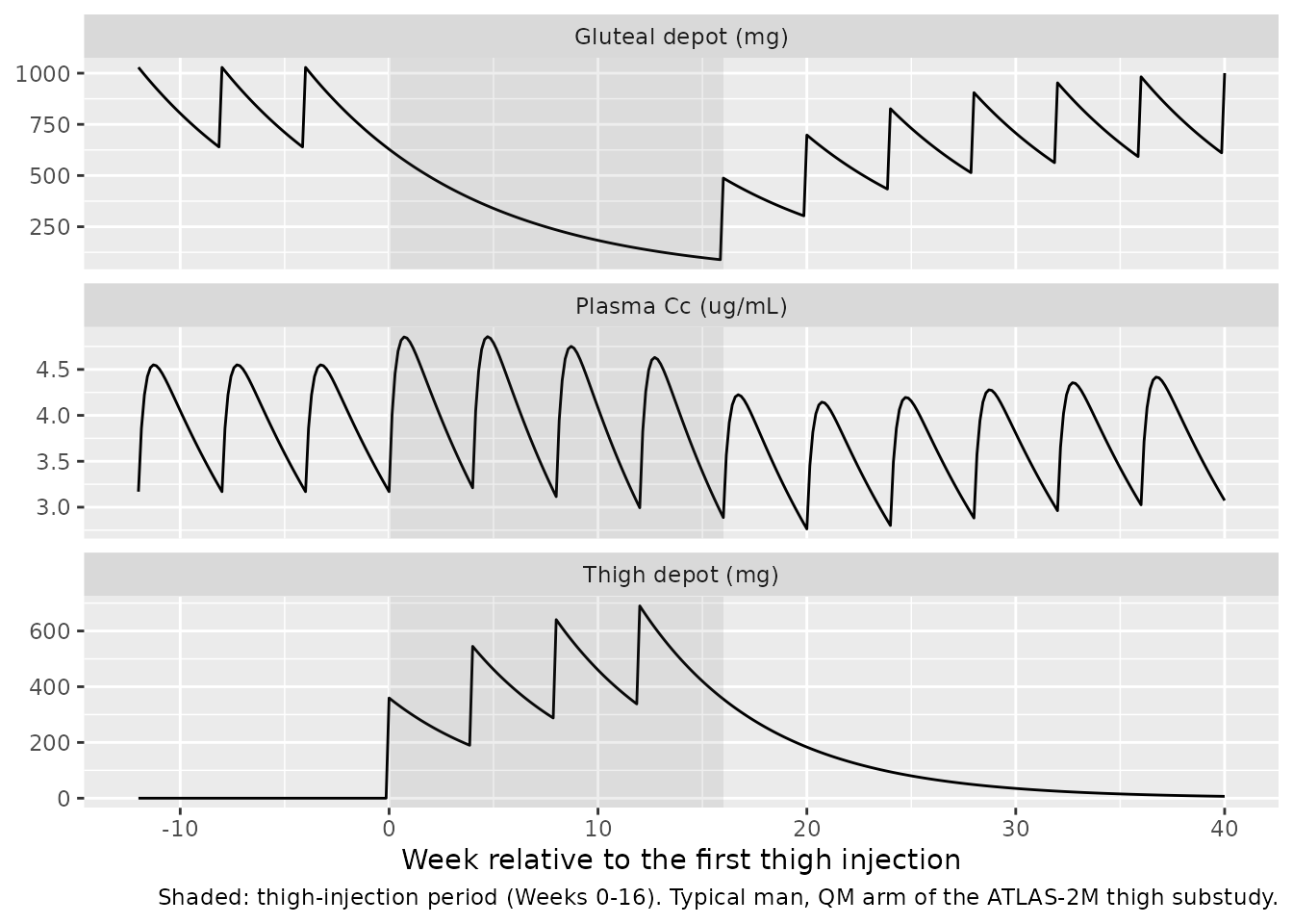
This scenario is why the model needs two IM depots. It follows the QM arm of the substudy for a typical 76.6 kg man. He first receives monthly gluteal injections (600 mg, then 400 mg) until steady state, with the last at Week -4. Thigh injections of 400 mg follow on Day 1 and at Weeks 4, 8 and 12, and gluteal injections resume at Week 16. The amount left in the gluteal depot drains with its 5.7-week half-life while the thigh depot fills and empties faster.
week <- 168
# Event times start at the first gluteal injection (Week -160) so that none
# is negative; `t0` shifts them back for plotting.
t0 <- 160 * week
gluteal_before <- seq(-160 * week, -4 * week, by = 4 * week)
thigh <- c(0, 4, 8, 12) * week
gluteal_after <- seq(16 * week, 40 * week, by = 4 * week)
doses_sw <- bind_rows(
  tibble(time = gluteal_before, cmt = "depot_im_gluteal"),
  tibble(time = thigh, cmt = "depot_im_thigh"),
  tibble(time = gluteal_after, cmt = "depot_im_gluteal")
) |>
  mutate(amt = ifelse(time == min(time), 600, 400), evid = 1L, time = time + t0)
obs_sw <- tibble(time = t0 + seq(-12 * week, 40 * week, by = 24), amt = 0, evid = 0L, cmt = "central")
ev_sw <- bind_rows(doses_sw, obs_sw) |>
  arrange(time, desc(evid)) |>
  mutate(id = 1L, WT = 76.6, SEXF = 0, BMI = 25.4, SMOKE = 0, INJ_SPLIT = 0, NEEDLE_LEN_IN = 1.5)
sim_sw <- rxode2::rxSolve(rxode2::zeroRe(mod), events = ev_sw, returnType = "data.frame") |>
  mutate(time = time - t0) |>
  dplyr::filter(time >= -12 * week)
#> ℹ parameter labels from comments will be replaced by 'label()'
#> ℹ omega/sigma items treated as zero: 'etalka_thigh', 'etalfdepot_thigh', 'etalka_gluteal', 'etalka_oral', 'etalfdepot_oral', 'etalcl', 'etalvc'

# Mass in the two IM depots, and plasma concentration
sim_sw |>
  transmute(
    week = time / week,
    `Gluteal depot (mg)` = depot_im_gluteal,
    `Thigh depot (mg)` = depot_im_thigh,
    `Plasma Cc (ug/mL)` = Cc
  ) |>
  tidyr::pivot_longer(-week) |>
  ggplot(aes(week, value)) +
  geom_line() +
  annotate("rect", xmin = 0, xmax = 16, ymin = -Inf, ymax = Inf, alpha = 0.1) +
  facet_wrap(~name, ncol = 1, scales = "free_y") +
  labs(
    x = "Week relative to the first thigh injection",
    y = NULL,
    caption = "Shaded: thigh-injection period (Weeks 0-16). Typical man, QM arm of the ATLAS-2M thigh substudy."
  )
# Both depots hold drug at the same time during the thigh period.
overlap <- dplyr::filter(sim_sw, time > 0, time < 16 * week)
stopifnot(all(overlap$depot_im_gluteal > 1), all(overlap$depot_im_thigh[overlap$time > 1] > 1))
During the thigh period, each dose is absorbed faster but is 10% less bioavailable than a gluteal dose. Faster absorption raises the peaks relative to the troughs, and lower bioavailability lowers the average concentration. The figure shows the net effect for a typical man.
Assumptions and deviations
- Women’s half-lives in the Results. Han 2024 quotes 6.4 weeks (thigh) and 10.6 weeks (gluteal) for women. The Table 2 parameters give 6.7 and 11.5 weeks; Han 2022 itself quotes 11.5 weeks for the gluteal value. Han 2024’s two figures imply KA values 34.5% and about 47% below the men’s values. The 34.5% matches the post-hoc sex difference in KA thigh that the Results report from Figure 3A. The quoted half-lives therefore appear to come from empirical post-hoc estimates in this cohort, not from the typical-value equation. They are derived quantities, so no parameter is affected. The package keeps the published equation, and the values are shown but not asserted above. The men’s values reproduce exactly.
-
Structure of the thigh rate. The main text gives
the typical-value equation
KA thigh = 0.0002527 + 0.00073 x (covariates). The Discussion could be read as adding the increment to each person’s own gluteal rate. The Supplemental Table settles the question: the final model isTV_KA3 = TV_KA2 + THETA1withKA3 = TV_KA3 * EXP(ETA). The rejectedKA3 = KA2 + DKAform fitted 6.0-12.8 OFV points worse. The thigh rate therefore carries its own eta, and the gluteal eta does not enter it. Because the typical thigh rate is a sum, it has no log-scale fixed effect. For that reasonetalka_thighhas nolka_thighpartner, and the convention check flags it. The increment isdka_thighon the natural scale. -
Inherited covariate effects on the thigh rate. The
sex, BMI, split and needle-length factors reach the thigh rate only
through the typical gluteal value. Han 2024 had no split thigh
injections, and only 3 of 366 used a needle other than 1.5 inches, so
these two factors were never tested for the thigh. One
INJ_SPLIT/NEEDLE_LEN_INcolumn serves both IM depots. - Fixed values not reprinted in Han 2024. KAoral, the body-weight exponents, the smoking effect, the gluteal / oral / CL / V2 IIV and the residual error do not appear in Han 2024 Table 2. They are read from Han 2022 Table 3 under the footnote that fixes every non-thigh parameter to that model. The residual error is treated as fixed as well. Han 2024 does not print it.
- IIV scale and covariances. IIV percentages are read as log-normal CVs, omega^2 = log(1 + CV^2). Thigh bioavailability uses a log-normal eta, like the oral F in Han 2022; Han 2024 does not print the form. The Methods say the four absorption and bioavailability etas were estimated separately. Han 2022’s covariances among KA gluteal, CL/F and V2/F were not published, so the whole block is diagonal.
- Body-weight reference. The fixed Han 2022 parameters are centred at 76.6 kg, not at the Han 2024 median of 75.75 kg.
- Covariate cohort. The paper resampled the covariates of real subjects for each subgroup. That table is not public, so the cohort here is synthetic, with one BMI distribution for both sexes. Months are 4 weeks.
-
HIV status. HIV status was screened on the thigh
parameters and not retained (Results), so it appears only in
covariatesDataExcluded.