Amoxicillin in breast milk (Baklouti 2026)
Source:vignettes/articles/Baklouti_2026_amoxicillin.Rmd
Baklouti_2026_amoxicillin.RmdModel and source
#> ℹ parameter labels from comments will be replaced by 'label()'Citation: Baklouti S, Rigourd V, Panchaud A, Nordeng H, Allegaert K, Annaert P, Huang MC, Monfort A, Guidi M, Gandia P. Population pharmacokinetic modelling of amoxicillin in human breast milk - A contribution from the ConcePTION project. Br J Clin Pharmacol. 2026;92(6):1833-1844. doi:10.1002/bcp.70434. All parameter values are the final estimates of Table 3; the ODE system and the Vmilk = Vc assumption are the display equations and prose of Results section 3.2 (pp. 1836-1837), and the model topology is Figure 1.
Description: Population PK model of oral amoxicillin in breastfeeding women, describing maternal plasma and breast-milk concentrations simultaneously. A gastrointestinal depot feeds a central (plasma) compartment by first-order absorption; the central compartment is drained both by first-order systemic elimination and by a UNIDIRECTIONAL first-order transfer into a breast-milk compartment, and milk is cleared by its own first-order loss constant. Nothing returns from milk to plasma: the authors tested a bidirectional peripheral-milk parameterisation and it failed to converge. The milk volume is not identifiable from the data and was fixed equal to the central volume, so the milk state is scaled by V/F. Because the milk loss constant runs continuously rather than only at feeds, the model understates milk amounts between feeds and is therefore a conservative (low) estimator of the relative infant dose; the authors flag this as its main structural limitation. Inter-individual variability on all five structural parameters, separate proportional residual errors for plasma and for milk, and no retained covariates.
Article: https://doi.org/10.1002/bcp.70434
Supplement (Appendix S1, the LC-MS/MS validation report for amoxicillin in milk; it contains no model parameters).
This is the first population PK model of amoxicillin developed in
breastfeeding women, and it is the amoxicillin arm of the European
ConcePTION consortium. The consortium’s cetirizine model is
modellib("Melander_2025_cetirizine").
Population
pop <- readModelDb("Baklouti_2026_amoxicillin")()$population
str(pop, max.level = 1)
#> List of 15
#>  $ species        : chr "human"
#>  $ n_subjects     : num 25
#>  $ n_studies      : num 1
#>  $ n_observations : num 150
#>  $ age_mean       : chr "35 years"
#>  $ weight_mean    : chr "64.9 kg"
#>  $ height_mean    : chr "164.5 cm"
#>  $ sex_female_pct : num 100
#>  $ renal_function : chr "Normal; CKD-EPI eGFR mean 114.7 mL/min/1.73 m^2 (SD 8.5, CV 7.4%). The narrow spread is why no renal covariate "| __truncated__
#>  $ disease_state  : chr "Breastfeeding women treated with oral immediate-release amoxicillin, with or without clavulanic acid, for at le"| __truncated__
#>  $ dose_range     : chr "Oral immediate-release amoxicillin 1 g twice daily (n = 6) or 1 g three times daily (n = 19); mean total daily "| __truncated__
#>  $ regions        : chr "France (recruited from the lactarium of Necker-Enfants Malades Hospital, Paris). EudraCT 2021-002247-30; French"| __truncated__
#>  $ infant_partner : chr "One breastfed infant per mother, all over 4 weeks old: 12 male / 13 female, mean postnatal age 5.5 months (SD 4"| __truncated__
#>  $ feeding_pattern: chr "Mothers reported a mean of 9 breastfeeds per day (SD 4, CV 47%; Table 1). The steady-state Monte Carlo simulati"| __truncated__
#>  $ notes          : chr "Baseline demographics from Baklouti 2026 Tables 1 and 2. Three blood and three milk samples per mother (75 + 75"| __truncated__
Twenty-five French breastfeeding mothers (mean age 35 years, mean weight 64.9 kg, mean CKD-EPI eGFR 114.7 mL/min/1.73 m^2) taking oral immediate-release amoxicillin 1 g twice daily (n = 6) or 1 g three times daily (n = 19) for at least two days, i.e. at steady state. Each contributed three plasma and three milk samples within a single dosing interval, nominally at 15-30 min, 1-2 h and 3-4 h post-dose, giving 75 + 75 = 150 observations (Baklouti 2026 Tables 1-2 and Results section 3.1). Milk was collected as roughly 20 mL of foremilk with an electric pump without emptying the breast; because amoxicillin is water-soluble and concentrates in low-fat foremilk, the authors describe this as a deliberate worst-case sampling scheme for milk exposure.
Source trace
Every value below is a final estimate from Baklouti 2026
Table 3. The per-parameter origin is also recorded as
an in-file comment beside each ini() entry in
inst/modeldb/specificDrugs/Baklouti_2026_amoxicillin.R.
| Equation / parameter | Value | Source location |
|---|---|---|
dG/dt = -ka*G, G(0) = F*D
|
– | Results 3.2, display equations p. 1836; Figure 1 |
dX/dt = ka*G - ke*X - kmilk*X |
– | Results 3.2, display equations p. 1836; Figure 1 |
dM/dt = kmilk*X - kmilk_e*M |
– | Results 3.2, display equations p. 1836; Figure 1 |
C(t) = X(t)/Vc |
– | Results 3.2, display equation p. 1836 |
Vmilk = Vc |
identity | Results 3.2, p. 1837 (“arbitrarily set to a value identical to that of the systemic compartment”) |
lka |
0.17 1/h | Table 3, k a (h-1), RSE 39.9%, 95%CI 0.085-0.35 |
lvc |
82.38 L | Table 3, V/F (L), RSE 11.0%, 95%CI 66.46-102.1 |
lkel |
0.31 1/h | Table 3, K e (h-1), RSE 23.1%, 95%CI 0.2-0.48 |
lk_central_milk |
0.028 1/h | Table 3, K milk (h-1), RSE 12.5%, 95%CI
0.022-0.036 |
lkeff_milk |
0.33 1/h | Table 3, K milk_e (h-1), RSE 19.4%, 95%CI
0.23-0.48 |
etalka |
0.37^2 | Table 3, IIV k a (se), RSE 44.2% |
etalvc |
0.086^2 | Table 3, IIV V/F (se), RSE 47.7% |
etalkel |
0.49^2 | Table 3, IIV K e (se), RSE 24.9% |
etalk_central_milk |
0.11^2 | Table 3, IIV K milk (se), RSE 64.8% |
etalkeff_milk |
0.38^2 | Table 3, IIV K milk_e (se), RSE 28.3% |
propSd (plasma) |
0.48 | Table 3, b1 (se), RSE 10.9% |
propSd_Cmilk (milk) |
0.26 | Table 3, b2 (se), RSE 11.3% |
The display equations do not survive plain-text extraction of the
PDF, and the publisher’s symbol font encodes minus and multiplication as
C0 control bytes, so the ODE signs above were recovered from the PDF
with pdftotext -layout and cat -A. The sign
that matters is on kmilk: it is subtracted from the central
compartment as well as added to milk, so transfer into milk is a genuine
elimination pathway for plasma and total plasma loss is
ke + kmilk = 0.338 1/h.
mod$state
#> [1] "depot"   "central" "milk"
Validation 1 – the steady-state milk:plasma AUC ratio is a closed form
Integrating the milk ODE over a complete steady-state dosing interval makes the milk state return to where it started, so the accumulation term vanishes:
0 = kmilk * integral(central) - kmilk_e * integral(milk)Because the model sets Vmilk = Vc, dividing through by
that common volume turns the amount integrals into concentration AUCs
and gives a ratio free of ka, ke and
Vc altogether:
AUC(milk) / AUC(plasma) = kmilk / kmilk_eThat is a zero-parameter falsifier for the whole extraction. Baklouti 2026 Table 4 reports a simulated milk/plasma AUC ratio with median 8.5% and quartiles 6.6-11.1%.
theta <- c(kmilk = 0.028, kmilk_e = 0.33)
omega <- c(kmilk = 0.11, kmilk_e = 0.38)   # Table 3 IIV, read as log-scale SDs

ratio_median <- theta[["kmilk"]] / theta[["kmilk_e"]]

# The per-subject ratio is a ratio of two independent lognormals, so it is
# itself lognormal: its median is the ratio of the medians and its log-scale
# SD is the root-sum-square of the two omegas.
sd_log  <- sqrt(sum(omega^2))
ratio_q <- ratio_median * exp(qnorm(c(0.25, 0.75)) * sd_log)

data.frame(
  Quantity  = c("Median", "First quartile", "Third quartile"),
  Predicted = sprintf("%.2f%%", 100 * c(ratio_median, ratio_q)),
  Published = c("8.5%", "6.6%", "11.1%")
) |>
knitr::kable(caption = "Closed-form milk/plasma AUC ratio vs Baklouti 2026 Table 4.")| Quantity | Predicted | Published |
|---|---|---|
| Median | 8.48% | 8.5% |
| First quartile | 6.50% | 6.6% |
| Third quartile | 11.08% | 11.1% |
The agreement is essentially exact, and it is a strong test in both
directions: it confirms the two milk rate constants, the
Vmilk = Vc identity, and the unidirectional topology at
once. It also settles a transcription question that Table 3 leaves open
– whether the IIV column holds standard deviations or
variances. Reading them as variances moves the
predicted quartiles to 5.3-13.6%, well outside the published
6.6-11.1%:
sd_if_variances <- sqrt(sum(omega))   # counterfactual: treat 0.11 / 0.38 as variances

data.frame(
  Reading = c("IIV are log-scale SDs (used here)", "IIV are variances"),
  Q1 = sprintf("%.2f%%", 100 * ratio_median * exp(qnorm(0.25) * c(sd_log, sd_if_variances))),
  Q3 = sprintf("%.2f%%", 100 * ratio_median * exp(qnorm(0.75) * c(sd_log, sd_if_variances))),
  Published = "6.6% - 11.1%"
) |>
knitr::kable(caption = "The published IQR discriminates between the two readings of Table 3's IIV column.")| Reading | Q1 | Q3 | Published |
|---|---|---|---|
| IIV are log-scale SDs (used here) | 6.50% | 11.08% | 6.6% - 11.1% |
| IIV are variances | 5.29% | 13.60% | 6.6% - 11.1% |
The Discussion independently corroborates the SD reading: it quotes
“a mean ka of 0.17 h-1 (CV = 37%)” against Table 3’s
IIV k a of 0.37.
Virtual cohort and steady-state simulation
The model carries no covariates, so a cohort needs only the random effects. Table 4’s simulations use the maximum recommended maintenance dose from the summary of product characteristics, 2 g every 8 h (6 g/day). Dosing runs for five days so that even the slowest-absorbing and slowest-eliminating subjects are at steady state before the analysis interval.
Both Cc and Cmilk are declared endpoints of
this model, so rxode2 returns each of them at every observation row and
a single observation grid is enough.
Observation rows must name a declared endpoint
(cmt = "Cc"), not an ODE state. This model has two error
models, so its endpoints occupy compartments 4 and 5 and rxode2 rejects
an observation that maps anywhere else: cmt = "central",
cmt = "milk", cmt = 2, a bare
dvid = 1L and an event table with no cmt at
all each fail with
'dvid'->'cmt' on observation record or on a undefined compartment.
This is the declared-endpoint case, which is legal and does not renumber
anything – it is not the “referencing an algebraic observable injects a
cmt() slot” trap, because Cc here is already a
slot.
rxode2::rxSetSeed(20260902)

n_sub    <- 200        # per-arm cap; ample for this check
tau      <- 8          # h
n_dose   <- 15         # five days of q8h dosing
ss_start <- (n_dose - 1) * tau
ss_end   <- ss_start + tau

ev <- rxode2::et(amt = 2000, ii = tau, addl = n_dose - 1, cmt = "depot") |>
  rxode2::et(seq(ss_start, ss_end, by = 0.05), cmt = "Cc")

sim <- rxode2::rxSolve(
  mod, ev, nSub = n_sub,
  # rxode2's automatic ODE -> linCmt conversion corrupts multi-output models
  useLinCmt = FALSE
) |>
  as.data.frame() |>
  # a single-subject event table replicated with nSub names the subject
  # index `sim.id`; rename it so PKNCA and the plots can use `id`
  dplyr::rename(id = sim.id)

str(sim[, c("id", "time", "Cc", "Cmilk", "k_central_milk", "keff_milk")])
#> 'data.frame':    32200 obs. of  6 variables:
#>  $ id            : int  1 1 1 1 1 1 1 1 1 1 ...
#>  $ time          : num  112 112 112 112 112 ...
#>  $ Cc            : num  3.33 3.52 3.7 3.88 4.05 ...
#>  $ Cmilk         : num  0.208 0.207 0.206 0.205 0.204 ...
#>  $ k_central_milk: num  0.0217 0.0217 0.0217 0.0217 0.0217 ...
#>  $ keff_milk     : num  0.467 0.467 0.467 0.467 0.467 ...
Cc and Cmilk above are individual
predictions (IPRED); no residual error is added, which is what the
closed-form checks below require.
sim |>
  dplyr::select(id, time, Plasma = Cc, Milk = Cmilk) |>
  tidyr::pivot_longer(c(Plasma, Milk), names_to = "Matrix", values_to = "conc") |>
  dplyr::mutate(tad = time - ss_start) |>
  dplyr::group_by(Matrix, tad) |>
  dplyr::summarise(
    med = median(conc), lo = quantile(conc, 0.05), hi = quantile(conc, 0.95),
    .groups = "drop"
  ) |>
  ggplot2::ggplot(ggplot2::aes(tad, med, ymin = lo, ymax = hi, fill = Matrix, colour = Matrix)) +
  ggplot2::geom_ribbon(alpha = 0.25, colour = NA) +
  ggplot2::geom_line(linewidth = 0.8) +
  ggplot2::scale_y_log10() +
  ggplot2::labs(x = "Time after dose (h)", y = "Amoxicillin concentration (mg/L)") +
  ggplot2::theme_bw()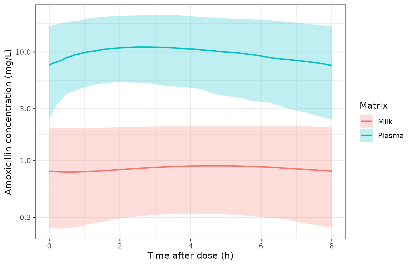
Simulated steady-state amoxicillin concentrations in maternal plasma and breast milk over one 8 h dosing interval at 2 g q8h (200 subjects; median and 5th-95th percentiles of the individual predictions). Milk concentrations sit roughly an order of magnitude below plasma and are visibly delayed and flattened relative to it, the behaviour shown by the prediction-corrected VPCs of Figure 4 of Baklouti 2026.
Validation 2 – PKNCA over the steady-state interval
nca_conc <- sim |>
  dplyr::select(id, time, Plasma = Cc, Milk = Cmilk) |>
  tidyr::pivot_longer(c(Plasma, Milk), names_to = "Matrix", values_to = "conc") |>
  dplyr::filter(!is.na(conc))

nca_dose <- nca_conc |>
  dplyr::distinct(id, Matrix) |>
  dplyr::mutate(time = ss_start, dose = 2000)

conc_obj <- PKNCA::PKNCAconc(nca_conc, conc ~ time | Matrix + id,
                             concu = "mg/L", timeu = "h")
dose_obj <- PKNCA::PKNCAdose(nca_dose, dose ~ time | Matrix + id,
                             doseu = "mg")

intervals <- data.frame(
  start = ss_start, end = ss_end,
  cmax = TRUE, tmax = TRUE, cmin = TRUE, auclast = TRUE, cav = TRUE
)

nca_res <- PKNCA::pk.nca(PKNCA::PKNCAdata(conc_obj, dose_obj, intervals = intervals))
nca_tab <- as.data.frame(nca_res)

nca_wide <- nca_tab |>
  dplyr::filter(PPTESTCD %in% c("cmax", "tmax", "cmin", "auclast", "cav")) |>
  tidyr::pivot_wider(id_cols = c(id, Matrix), names_from = PPTESTCD, values_from = PPORRES)

head(nca_wide)
#> # A tibble: 6 × 7
#>      id Matrix auclast  cmax  cmin  tmax   cav
#>   <int> <chr>    <dbl> <dbl> <dbl> <dbl> <dbl>
#> 1     1 Milk      1.97 0.276 0.204  4    0.246
#> 2     2 Milk      5.78 0.760 0.672  4.75 0.722
#> 3     3 Milk      4.69 0.629 0.526  4.45 0.586
#> 4     4 Milk     10.7  1.42  1.22   4.7  1.33
#> 5     5 Milk      3.90 0.548 0.403  4.05 0.488
#> 6     6 Milk     12.0  1.56  1.43   5    1.51
nca_wide |>
  dplyr::group_by(Matrix) |>
  dplyr::summarise(
    cmax = median(cmax), tmax = median(tmax), cmin = median(cmin),
    cav = median(cav), auclast = median(auclast), .groups = "drop"
  ) |>
  dplyr::rename(
    "Matrix"            = Matrix,
    "Cmax (mg/L)"       = cmax,
    "Tmax (h)"          = tmax,
    "Cmin (mg/L)"       = cmin,
    "Cavg (mg/L)"       = cav,
    "AUC0-tau (mg*h/L)" = auclast
  ) |>
knitr::kable(digits = 3, caption = "Median steady-state NCA parameters at 2 g q8h, by matrix.")| Matrix | Cmax (mg/L) | Tmax (h) | Cmin (mg/L) | Cavg (mg/L) | AUC0-tau (mg*h/L) |
|---|---|---|---|---|---|
| Milk | 0.838 | 4.65 | 0.714 | 0.786 | 6.289 |
| Plasma | 10.301 | 2.70 | 6.550 | 8.880 | 71.040 |
Baklouti 2026 reports no NCA table of its own – the paper’s only exposure summaries are the milk/plasma ratios and the relative infant dose of Table 4 – so the NCA is validated against the model’s own closed form rather than against a published NCA table.
The per-subject AUC-ratio identity
For each subject the two sides of the identity use the same
drawn parameters, so the only difference is trapezoidal and integration
error. That makes a tight bound the correct assertion here, unlike the
cohort-versus-publication comparison that follows. Note that the
prediction is each subject’s own
k_central_milk / keff_milk, not the population value.
subject_k <- sim |>
  dplyr::group_by(id) |>
  dplyr::summarise(k_ratio = first(k_central_milk) / first(keff_milk), .groups = "drop")

ratio_chk <- nca_wide |>
  dplyr::select(id, Matrix, auclast) |>
  tidyr::pivot_wider(names_from = Matrix, values_from = auclast) |>
  dplyr::left_join(subject_k, by = "id") |>
  dplyr::mutate(
    observed = Milk / Plasma,
    pct_diff = 100 * (observed - k_ratio) / k_ratio
  )

summary(ratio_chk$pct_diff)
#>       Min.    1st Qu.     Median       Mean    3rd Qu.       Max.
#> -0.0227078  0.0007894  0.0013469  0.0011479  0.0019255  0.0108162

stopifnot(
  # Solve against its own closed form: pure numerical error, so bound tightly.
  max(abs(ratio_chk$pct_diff)) < 0.5
)
Cohort ratio against the published Table 4
q_sim <- quantile(ratio_chk$observed, c(0.25, 0.5, 0.75))

data.frame(
  Statistic = c("First quartile", "Median", "Third quartile"),
  Simulated = sprintf("%.2f%%", 100 * q_sim),
  Published = c("6.6%", "8.5%", "11.1%")
) |>
knitr::kable(caption = "Simulated milk/plasma AUC ratio vs Baklouti 2026 Table 4 (simulated, random breastfeeding).")| Statistic | Simulated | Published |
|---|---|---|
| First quartile | 6.38% | 6.6% |
| Median | 8.51% | 8.5% |
| Third quartile | 11.36% | 11.1% |
stopifnot(
  # Centre: a mis-transcribed rate constant moves this by tens of percent.
  abs(100 * q_sim[["50%"]] - 8.5) < 1.5,
  # Envelope: robust quartiles rather than extremes, so the check does not
  # depend on which subjects land in the tails of a randomly drawn cohort.
  abs(100 * q_sim[["25%"]] - 6.6) < 2,
  abs(100 * q_sim[["75%"]] - 11.1) < 2.5
)
Validation 3 – milk/plasma concentration ratio
Table 4 also reports a milk/plasma concentration ratio – median 4.8%, quartiles 4.1-5.2%, range 3.3-5.4% – described as being sampled at simulated feeding times drawn across the day. For this model structure that quantity is tightly constrained by the AUC ratio, because the milk profile is a smoothed and delayed copy of the plasma profile rather than an independently shaped curve.
tv <- rxode2::rxSolve(rxode2::zeroRe(mod), ev, useLinCmt = FALSE) |> as.data.frame()
#> ℹ omega/sigma items treated as zero: 'etalka', 'etalvc', 'etalkel', 'etalk_central_milk', 'etalkeff_milk'
tv$ratio <- 100 * tv$Cmilk / tv$Cc

cohort_ratio <- sim |>
  dplyr::mutate(ratio = 100 * Cmilk / Cc) |>
  dplyr::filter(is.finite(ratio)) |>
  dplyr::pull(ratio)

data.frame(
  Source = c(
    "Typical subject, across the dosing interval",
    "Cohort (200 subjects, all interval times)",
    "Published simulated concentration ratio",
    "Published simulated AUC ratio",
    "Published MEASURED concentration ratio"
  ),
  Q1     = c(sprintf("%.1f%%", quantile(tv$ratio, 0.25)), sprintf("%.1f%%", quantile(cohort_ratio, 0.25)), "4.1%", "6.6%", "4.5%"),
  Median = c(sprintf("%.1f%%", median(tv$ratio)),         sprintf("%.1f%%", median(cohort_ratio)),         "4.8%", "8.5%", "6.0%"),
  Q3     = c(sprintf("%.1f%%", quantile(tv$ratio, 0.75)), sprintf("%.1f%%", quantile(cohort_ratio, 0.75)), "5.2%", "11.1%", "9.6%")
) |>
knitr::kable(caption = "Milk/plasma concentration ratio produced by the packaged model, against the three ratios of Baklouti 2026 Table 4.")| Source | Q1 | Median | Q3 |
|---|---|---|---|
| Typical subject, across the dosing interval | 7.6% | 8.4% | 9.5% |
| Cohort (200 subjects, all interval times) | 6.4% | 8.5% | 11.6% |
| Published simulated concentration ratio | 4.1% | 4.8% | 5.2% |
| Published simulated AUC ratio | 6.6% | 8.5% | 11.1% |
| Published MEASURED concentration ratio | 4.5% | 6.0% | 9.6% |
The model’s concentration ratio sits at roughly 8.4-8.8%, i.e. it tracks the AUC ratio closely, and it falls inside the interquartile range of the paper’s own measured milk/plasma ratio (4.5-9.6%, median 6.0%). It does not reproduce the paper’s simulated concentration ratio of 4.8%, which is about half the model’s value.
That row appears to be internally inconsistent with the rest of Table
4 rather than a transcription error on our side. The simulated
concentration ratio and the simulated AUC ratio are reported as coming
from the same 10 000-draw simulation of the same model, yet for a
structure in which milk is a linear first-order filter of plasma the two
cannot differ by a factor of two: averaging Cmilk/Cc over
the interval and dividing the two AUCs give nearly the same number, as
the typical-subject row above shows (8.4% versus the closed-form
8.485%). The published concentration-ratio row is also implausibly tight
– a full min-max of 3.3-5.4% across 10 000 draws, narrower than its own
interquartile range for the AUC ratio, despite the two milk rate
constants carrying 11% and 38% inter-individual variability. No
assertion is made against that row; the AUC ratio is the reproducible
gate.
# Averaging the concentration ratio over the interval and taking the ratio of
# the AUCs are two routes to the same number for this structure.
auc_tv <- c(
  milk   = sum(diff(tv$time) * (head(tv$Cmilk, -1) + tail(tv$Cmilk, -1)) / 2),
  plasma = sum(diff(tv$time) * (head(tv$Cc, -1)    + tail(tv$Cc, -1))    / 2)
)

data.frame(
  Route = c("Median of Cmilk/Cc over the interval", "AUC(milk) / AUC(plasma)", "Closed form kmilk / kmilk_e"),
  Value = sprintf("%.3f%%", c(median(tv$ratio), 100 * auc_tv[["milk"]] / auc_tv[["plasma"]], 100 * ratio_median))
) |>
knitr::kable(caption = "Typical subject: the concentration ratio and the AUC ratio are the same quantity for this model.")| Route | Value |
|---|---|
| Median of Cmilk/Cc over the interval | 8.427% |
| AUC(milk) / AUC(plasma) | 8.485% |
| Closed form kmilk / kmilk_e | 8.485% |
Validation 4 – relative infant dose
# Relative infant dose: the infant's weight-adjusted daily dose as a percentage
# of the mother's, assuming the standard 150 mL/kg/day milk intake
# (Methods section 2.4).
milk_intake <- 0.15                  # L/kg/day
maternal_wt <- 65                    # kg (Table 4 note)
maternal_dd <- 3 * 2000              # mg/day at 2 g q8h

rid <- nca_wide |>
  dplyr::filter(Matrix == "Milk") |>
  dplyr::mutate(
    infant_dose = cav * milk_intake,           # mg/kg/day
    maternal_pk = maternal_dd / maternal_wt,   # mg/kg/day
    rid_pct     = 100 * infant_dose / maternal_pk
  )

data.frame(
  Statistic = c("Median", "Third quartile", "Maximum"),
  Simulated = sprintf("%.3f%%", c(median(rid$rid_pct), quantile(rid$rid_pct, 0.75), max(rid$rid_pct))),
  Published = c("0.03%", "0.03%", "0.07%")
) |>
knitr::kable(caption = "Relative infant dose at 2 g q8h vs Baklouti 2026 Table 4 (simulated, adult dosage).")| Statistic | Simulated | Published |
|---|---|---|
| Median | 0.128% | 0.03% |
| Third quartile | 0.196% | 0.03% |
| Maximum | 0.668% | 0.07% |
stopifnot(
  # The paper's clinical conclusion is that the RID sits far below the 2-3%
  # threshold at which breastfeeding is considered compatible. That conclusion
  # reproduces with a wide margin even though the exact published value does
  # not -- see Assumptions and deviations.
  median(rid$rid_pct) < 1,
  quantile(rid$rid_pct, 0.95) < 1
)
Computing the relative infant dose from the interval-average milk concentration gives roughly 0.1%, several times the published median of 0.03%, and it inherits the concentration-ratio discrepancy discussed above. Both figures are more than an order of magnitude below the 2-3% compatibility threshold, so the paper’s clinical conclusion – that amoxicillin is compatible with breastfeeding – is unaffected.
Assumptions and deviations
Milk volume.
Vmilkis fixed equal toVc(82.4 L). This is the authors’ own choice, made because milk volume was not identifiable and estimating it degraded the fit (Results section 3.2, p. 1837). It is not physiological – daily milk output averages about 2 L – and the Discussion defends it as avoiding over-parameterisation. Every milk concentration the model produces is therefore scaled by an apparent volume, not a real one. The milk/plasma ratio is nevertheless meaningful because the same volume divides both sides.IIV on V/F. Methods section 2.3 states that “IIV was included in ka, ke, kmilk and kmilk_e”, omitting V/F, but Table 3 tabulates
IIV V/F (se) 0.086with RSE 47.7% and a 95% CI of 0.038-0.2. A row carrying an RSE and a confidence interval is an estimated component, so Table 3 was taken as authoritative and the eta on V/F was retained. The Methods sentence appears to be simply incomplete.IIV scale. Table 3’s
IIVrows are labelled(se)without stating whether they hold standard deviations or variances. They are encoded here as log-scale standard deviations, squared into rxode2’s variance parameterisation. Two independent printed quantities confirm this: the published AUC-ratio interquartile range (Validation 1) and the Discussion’s “CV = 37%” againstIIV k a = 0.37.Rate-constant parameterisation. The paper estimates
keandV/Fas two separate parameters with an independent eta on each, so the model is encoded withlkelbeside an explicitlvcrather than being reparameterised tolcl+lvc. The clearance form is algebraically equivalent only ifetalcl = etalkel + etalvc, a correlated eta block the authors did not fit, so reparameterising would change the model.Continuous milk elimination.
keff_milkruns continuously, whereas milk is physically removed only at feeds. The authors flag this as the model’s main structural limitation and note that the drug amount in milk – and hence the relative infant dose – “would be higher if kmilk_e were set to zero between two consecutive feedings”. The packaged model reproduces the published structure rather than correcting it.Simulated concentration ratio and relative infant dose are not reproducible. The model reproduces Table 4’s simulated milk/plasma AUC ratio exactly (median and both quartiles), but gives about 8.5% where Table 4 reports 4.8% for the simulated concentration ratio, and about 0.1% where Table 4 reports 0.03% for the relative infant dose. Validation 3 shows the concentration-ratio row is inconsistent with the AUC-ratio row from the same simulation given this model structure, and its published spread (3.3-5.4% across 10 000 draws) is far too narrow for parameters carrying 11% and 38% inter-individual variability. Methods section 2.4 does not state how milk volume is apportioned per feed or whether the milk compartment is emptied at a feed, so the published accumulation cannot be reconstructed from the printed method. The Discussion contains a further figure that reconciles with neither – a “maximal daily intake of amoxicillin from our model (0.022 mg/day)”, corresponding to a relative infant dose near 0.004%. No parameter was tuned to close any of these gaps; the model reproduces the published estimates and the published AUC ratio, and the differences are reported as found.
Foremilk sampling. All milk observations are foremilk collected without emptying the breast, which the authors state overestimates concentrations relative to whole-feed milk. The model inherits that bias, which is conservative for a safety assessment.
No covariates. None of maternal age, weight, height, breastfeeding exclusivity, eGFR or albumin, nor infant age, weight or height, was retained. The Discussion attributes the null renal result to the narrow eGFR spread in the cohort (CV 7.4%) rather than to the absence of a relationship. All screened covariates are documented in the model file’s
covariatesDataExcluded.No published NCA table. The paper reports no NCA summary, so the NCA section is validated against the model’s closed form rather than a published table.