Meropenem (Fukumoto 2023)
Source:vignettes/articles/Fukumoto_2023_meropenem.Rmd
Fukumoto_2023_meropenem.RmdModel and source
- Citation: Fukumoto S, Ohbayashi M, Okada A, Kohyama N, Tamatsukuri T, Inoue H, Kato A, Kotani T, Sagara H, Dohi K, Kogo M. (2023). Population pharmacokinetic model and dosing simulation of meropenem using measured creatinine clearance for patients with sepsis. Ther Drug Monit 45(3):392-399. doi:10.1097/FTD.0000000000001040
- Description: Two-compartment IV population PK model for meropenem in 31 adults with sepsis in a Japanese emergency center / ICU (Fukumoto 2023). Clearance scales as a power function of the BSA-normalized MEASURED creatinine clearance obtained from an 8-hour timed urine collection, CL = 13.6 * (CRCL / 87.6)^0.66 L/h, centered on the cohort-median 87.6 mL/min/1.73 m^2. The measured CCr was the single retained covariate and outperformed Cockcroft-Gault CCr and eGFR, which underestimate renal function in septic patients with normal or augmented renal clearance. Interindividual variability was estimated on CL and V1 only; the random effects on Q and V2 were fixed at zero. Residual error is proportional.
- Article: https://doi.org/10.1097/FTD.0000000000001040
Fukumoto 2023 is a prospective observational population-PK study of meropenem in adults with sepsis, notable for measuring renal function directly by an 8-hour timed urine collection rather than estimating it with the Cockcroft-Gault (CG) equation. The paper’s two deliverables are (1) a two-compartment popPK model whose only retained covariate is the measured creatinine clearance on CL, and (2) a Monte Carlo dosing simulation that recommends prolonged and continuous infusions for patients with preserved or augmented renal clearance.
Population
Thirty-two adults with sepsis were enrolled at the emergency center or intensive care unit of Showa University Hospital (Tokyo, Japan) between June 2016 and August 2021; one patient met an exclusion criterion, leaving 31 analyzed. Exclusions were age under 18 years, hemodialysis, massive bleeding, pregnancy, and death during the urine collection.
Baseline characteristics from Fukumoto 2023 Table 1 (median (range)): age 72 (18-94) years, 25/31 male (19.4% female), weight 53.7 (35.3-91.7) kg, BSA 1.59 (1.26-2.01) m^2, BMI 22.2 (13.8-29.9) kg/m^2. Illness severity: SOFA score 8 (2-15) on admission and 6 (0-11) at blood collection; CRP 11.0 (0.72-41.0) mg/dL; WBC 13.0 (2.70-30.6) x 10^3/uL; albumin 2.10 (1.50-3.10) g/dL. Vasopressors were used in 9/31 (29%) and intravenous diuretics in 5/31 (16%), with a median daily intravenous fluid volume of 1000 (200-3900) mL.
Renal function spanned a deliberately broad range: measured CCr 87.6 (12.3-223) mL/min/1.73 m^2, CG-CCr 81.1 (14.0-246) mL/min, eGFR 86.0 (15.6-222) mL/min/1.73 m^2, and serum creatinine 0.69 (0.29-2.39) mg/dL. Eight patients (26%) had augmented renal clearance (CCr at or above 130 mL/min/1.73 m^2) and three (10%) had CCr at or below 30.
One hundred plasma samples were collected (2-5 per patient, median 2) within a single dosing interval after at least three doses, that is, at steady state, at predose (trough) and 0.5, 1, 2, 4 and 8 hours post-dose. Total meropenem was assayed by HPLC-UV at 300 nm with cefotaxime as internal standard, calibrated linearly over 0.1-80 mcg/mL. Estimation used Phoenix NLME 8.1 (FOCE-ELS); covariates were selected by stepwise forward addition (P < 0.05) and backward elimination (P < 0.01); validation used GOF plots, a prediction-corrected VPC, and a 1000-replicate bootstrap with a 100% success rate.
The same information is available programmatically via the model’s
population metadata
(readModelDb("Fukumoto_2023_meropenem")$population).
Source trace
Per-parameter origins are recorded inline in
inst/modeldb/specificDrugs/Fukumoto_2023_meropenem.R. The
table below collects them for review. Fukumoto 2023 Table 2 prints the
structural model directly in its row headings, so the equations and the
estimates share a source location.
| Equation / parameter | Value (RSE %) | Bootstrap median [95% CI] | Source location |
|---|---|---|---|
V1 = theta1, lvc -> exp(lvc) = 26.5
L |
26.5 (13.6) | 26.6 [21.4, 36.0] | Table 2, p. 395 |
CL = theta2 * (measured CCr / 87.6)^theta5,
lcl -> exp(lcl) = 13.6 L/h |
13.6 (5.04) | 13.6 [12.4, 15.2] | Table 2, p. 395 |
e_crcl_cl (theta5, power exponent) |
0.66 (11.9) | 0.67 [0.52, 0.84] | Table 2, p. 395 |
V2 = theta3, lvp -> exp(lvp) = 13.2
L |
13.2 (21.2) | 13.4 [9.51, 20.0] | Table 2, p. 395 |
Q = theta4, lq -> exp(lq) = 9.80
L/h |
9.80 (43.0) | 9.59 [2.29, 20.3] | Table 2, p. 395 |
etalvc = log(0.230^2 + 1) = 0.051538 |
IIV V1 23.0% CV (127) | 21.5% [0.0003, 56.7] | Table 2, p. 395 |
etalcl = log(0.221^2 + 1) = 0.047686 |
IIV CL 22.1% CV (32.4) | 21.1% [12.7, 27.7] | Table 2, p. 395 |
etalq ~ fixed(0), etalvp ~ fixed(0)
|
fixed at zero | n/a | Results “PPK Model”, p. 395 |
propSd = 0.194 |
Proportional 19.4% (13.1) | 18.4% [13.0, 23.4] | Table 2, p. 395 |
| Covariate centering value 87.6 mL/min/1.73 m^2 | cohort median measured CCr | n/a | Table 2 row heading, p. 395; Table 1, p. 394 |
| Measured CCr definition (BSA-normalized) | Equation 1 | n/a | Methods, p. 393 |
| Exponential IIV model; proportional residual error | n/a | n/a | Methods p. 394; Results p. 395 |
The eta-shrinkage reported for the final model was 41.4% for V1 and 7.75% for CL (Results, p. 395).
Virtual cohort
The paper’s Monte Carlo simulation dosed 10,000 virtual patients at
each of a grid of fixed creatinine-clearance values (30, 50, 70, 80, 85,
100, 130, 160 and 200 mL/min) with 1 or 2 g meropenem given over 0.5 h
(intermittent), 3 h (prolonged), 8 h or 12 h (continuous). Table 3 then
reports the probability of target attainment (PTA) for
50% T > MIC by renal-function band, and Figure
2 reports PTA for 100% T > MIC.
This vignette reproduces the same structure with 200 virtual patients per arm (see “Assumptions and deviations” for why 200 rather than 10,000, and for how the Table 3 bands are mapped onto single CCr values). Because Fukumoto 2023 retained no weight or demographic covariate, a virtual patient is fully specified by its measured CCr plus the two random effects on CL and V1, so no demographic distributions need to be assumed.
set.seed(20260728)

n_sub <- 200L

# Table 3 renal-function bands are represented by the highest (worst-case)
# CCr in each band; CCr 50 is added because Figure 2 reports 100% T > MIC
# PTAs at that exact value. See "Assumptions and deviations".
crcl_grid    <- c(50, 84, 99, 129, 159, 200)
infusion_grid <- c(0.5, 3, 8)

arm_defs <- tidyr::expand_grid(crcl = crcl_grid, infusion_h = infusion_grid) |>
  mutate(
    arm       = sprintf("CCr %g / %g-h infusion", crcl, infusion_h),
    id_offset = (row_number() - 1L) * n_sub
  )

dose_amt_mg <- 1000
tau_h       <- 8
dose_times  <- seq(0, 32, by = tau_h)   # five q8h doses; the 32-40 h interval is at steady state

build_arm <- function(crcl, infusion_h, arm, id_offset) {
  ids <- id_offset + seq_len(n_sub)

  dose_rows <- tidyr::expand_grid(id = ids, time = dose_times) |>
    mutate(evid = 1L, amt = dose_amt_mg, cmt = "central",
           rate = dose_amt_mg / infusion_h)

  # Dense grids over two dosing intervals at 0.025 h resolution, which gives
  # T > MIC to within 0.31% of the 8-hour interval. The 32-40 h window is the
  # terminal (steady-state) interval used throughout; the 8-16 h window is the
  # second dosing interval, used only for the sensitivity analysis in the
  # "100% T > MIC" section below.
  obs_rows <- tidyr::expand_grid(
    id   = ids,
    time = c(seq(8, 16, by = 0.025), seq(32, 40, by = 0.025))
  ) |>
    mutate(evid = 0L, amt = 0, cmt = "central", rate = 0)

  bind_rows(dose_rows, obs_rows) |>
    mutate(CRCL = crcl, arm = arm, infusion_h = infusion_h, crcl_val = crcl) |>
    arrange(id, time, desc(evid))
}

events <- purrr::pmap_dfr(arm_defs, build_arm)

stopifnot(nrow(arm_defs) * n_sub == dplyr::n_distinct(events$id))
Simulation
mod <- readModelDb("Fukumoto_2023_meropenem")

# `CRCL` is a model covariate, so rxode2 already returns it as an output
# column; listing it in `keep` too would produce duplicate column names.
# `drop_dup_cols()` additionally guards against rxode2 emitting the covariate
# column more than once, which it does in the `zeroRe()` + `omega = NA` path
# below; dplyr verbs refuse to operate on a frame with duplicate names.
drop_dup_cols <- function(df) df[, !duplicated(names(df)), drop = FALSE]

sim <- rxode2::rxSolve(
  mod,
  events = events,
  keep   = c("arm", "infusion_h", "crcl_val")
) |> as.data.frame() |> drop_dup_cols()
#> ℹ parameter labels from comments will be replaced by 'label()'
#> ℹ omega/sigma items treated as zero: 'etalq', 'etalvp'
A matching typical-value (random effects zeroed) run is used for the
concentration-time figures and for the closed-form clearance check.
omega = NA is passed alongside zeroRe()
because zeroRe() alone can still draw random effects when a
stochastic solve has already run in the same session.
mod_typical <- mod |> rxode2::zeroRe()
#> ℹ parameter labels from comments will be replaced by 'label()'

typ_events <- arm_defs |>
  select(crcl, infusion_h, arm) |>
  mutate(id = row_number()) |>
  tidyr::expand_grid(time = c(dose_times, seq(0, 48, by = 0.05))) |>
  distinct(id, crcl, infusion_h, arm, time) |>
  mutate(
    evid = if_else(time %in% dose_times, 1L, 0L),
    amt  = if_else(evid == 1L, dose_amt_mg, 0),
    cmt  = "central",
    rate = if_else(evid == 1L, dose_amt_mg / infusion_h, 0),
    CRCL = crcl
  ) |>
  arrange(id, time, desc(evid))

sim_typical <- rxode2::rxSolve(
  mod_typical,
  events = typ_events,
  omega  = NA,
  keep   = c("arm", "infusion_h", "crcl")
) |> as.data.frame() |> drop_dup_cols()
#> Warning: multi-subject simulation without without 'omega'
#> Warning: Cannot keep missing columns:
Concentration-time profiles across renal function
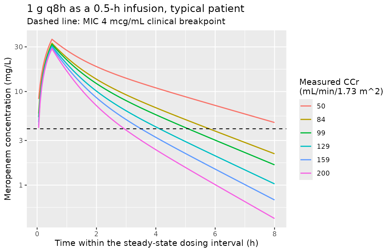
The figure below shows the typical-value steady-state profile for 1 g q8h given as a 0.5-hour intermittent infusion at each simulated creatinine clearance. It is the structural picture behind the paper’s central claim: as measured CCr rises the trough falls steeply, and by CCr 130-200 mL/min/1.73 m^2 the concentration spends much of the interval below the 4 mcg/mL clinical breakpoint (dashed line).
sim_typical |>
  filter(infusion_h == 0.5, time >= 32, time <= 40) |>
  mutate(time_in_interval = time - 32) |>
  ggplot(aes(time_in_interval, Cc, colour = factor(crcl))) +
  geom_line(linewidth = 0.7) +
  geom_hline(yintercept = 4, linetype = "dashed") +
  scale_y_log10() +
  labs(
    x = "Time within the steady-state dosing interval (h)",
    y = "Meropenem concentration (mg/L)",
    colour = "Measured CCr\n(mL/min/1.73 m^2)",
    title = "1 g q8h as a 0.5-h infusion, typical patient",
    subtitle = "Dashed line: MIC 4 mcg/mL clinical breakpoint"
  )
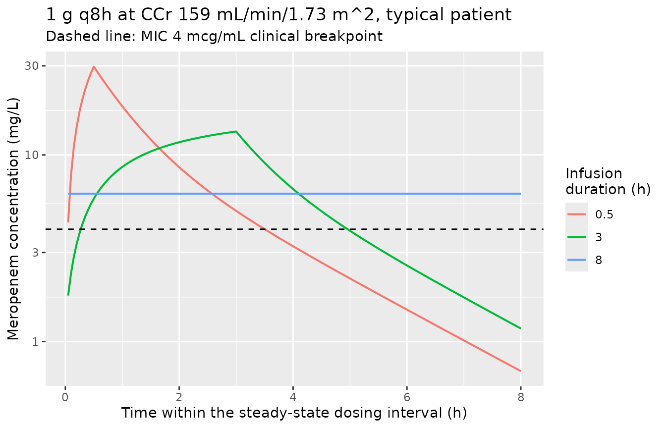
Extending the infusion trades peak concentration for time above the MIC, which is the mechanism behind the paper’s dosing recommendations. At CCr 159 mL/min/1.73 m^2 the 0.5-hour infusion drops below 4 mcg/mL well before the end of the interval, the 3-hour prolonged infusion is borderline, and the 8-hour continuous infusion holds a flat concentration above the breakpoint.
sim_typical |>
  filter(crcl == 159, time >= 32, time <= 40) |>
  mutate(time_in_interval = time - 32) |>
  ggplot(aes(time_in_interval, Cc, colour = factor(infusion_h))) +
  geom_line(linewidth = 0.7) +
  geom_hline(yintercept = 4, linetype = "dashed") +
  scale_y_log10() +
  labs(
    x = "Time within the steady-state dosing interval (h)",
    y = "Meropenem concentration (mg/L)",
    colour = "Infusion\nduration (h)",
    title = "1 g q8h at CCr 159 mL/min/1.73 m^2, typical patient",
    subtitle = "Dashed line: MIC 4 mcg/mL clinical breakpoint"
  )
PKNCA validation
Fukumoto 2023 reports no non-compartmental analysis of its own, so
there is no published NCA table to compare against. The NCA is instead
used as an internal consistency check with an exact analytical
reference: at steady state the area under the curve over a dosing
interval must equal Dose / CL, and the average
concentration must equal Dose / (CL * tau), where
CL = 13.6 * (CRCL / 87.6)^0.66. This validates the
covariate model, the units, and the infusion encoding
simultaneously.
NCA is run on the stochastic cohort over the 32-40 h steady-state
interval (thinned to a 0.1 h grid, which is ample for AUC). Because IIV
on CL is log-normal and AUC is a monotone function of CL, the
median simulated AUC should match
Dose / CL_typical up to Monte Carlo error.
nca_conc <- sim |>
  filter(infusion_h == 0.5, time >= 32, !is.na(Cc),
         abs(time / 0.1 - round(time / 0.1)) < 1e-8) |>
  mutate(treatment = sprintf("CCr %g", crcl_val)) |>
  select(id, time, Cc, treatment)

nca_dose <- events |>
  filter(infusion_h == 0.5, evid == 1L, time == max(dose_times)) |>
  mutate(treatment = sprintf("CCr %g", crcl_val)) |>
  select(id, time, amt, treatment)

conc_obj <- PKNCA::PKNCAconc(nca_conc, Cc ~ time | treatment + id,
                             concu = "mg/L", timeu = "hr")
dose_obj <- PKNCA::PKNCAdose(nca_dose, amt ~ time | treatment + id,
                             doseu = "mg")

intervals <- data.frame(
  start   = 32,
  end     = 40,
  cmax    = TRUE,
  cmin    = TRUE,
  tmax    = TRUE,
  auclast = TRUE,
  cav     = TRUE
)

nca_res <- PKNCA::pk.nca(PKNCA::PKNCAdata(conc_obj, dose_obj, intervals = intervals))
Population summary of the steady-state exposure metrics (median and 5th-95th percentiles across the 200 virtual patients per arm):
as.data.frame(nca_res$result) |>
  group_by(treatment, PPTESTCD) |>
  summarise(
    summary_value = sprintf("%.3g [%.3g, %.3g]",
                            median(PPORRES),
                            quantile(PPORRES, 0.05),
                            quantile(PPORRES, 0.95)),
    .groups = "drop"
  ) |>
  tidyr::pivot_wider(names_from = PPTESTCD, values_from = summary_value) |>
  rename(
    "Arm"                 = treatment,
    "Cmax (mg/L)"         = cmax,
    "Cmin (mg/L)"         = cmin,
    "Tmax (h)"            = tmax,
    "AUCtau (mg*h/L)"     = auclast,
    "Cavg (mg/L)"         = cav
  ) |>
knitr::kable(caption = "Steady-state NCA, 1 g q8h as a 0.5-h infusion. Median [5th, 95th percentile].")| Arm | AUCtau (mg*h/L) | Cavg (mg/L) | Cmax (mg/L) | Cmin (mg/L) | Tmax (h) |
|---|---|---|---|---|---|
| CCr 129 | 58.1 [39.3, 82.5] | 7.26 [4.91, 10.3] | 30.8 [23.5, 39.5] | 1.05 [0.34, 2.7] | 0.5 [0.5, 0.5] |
| CCr 159 | 47.8 [35.1, 70.3] | 5.98 [4.39, 8.78] | 29.3 [22.5, 38.9] | 0.654 [0.218, 2.04] | 0.5 [0.5, 0.5] |
| CCr 200 | 43.6 [30.4, 62.4] | 5.45 [3.81, 7.8] | 29.3 [21.5, 38.4] | 0.457 [0.16, 1.42] | 0.5 [0.5, 0.5] |
| CCr 50 | 104 [77.4, 149] | 13 [9.68, 18.7] | 36.9 [28.4, 47.7] | 4.44 [2.16, 8.85] | 0.5 [0.5, 0.5] |
| CCr 84 | 74.4 [51.9, 107] | 9.31 [6.48, 13.4] | 32.4 [24.3, 42.6] | 2.09 [0.76, 5.23] | 0.5 [0.5, 0.5] |
| CCr 99 | 67.6 [46.4, 95.7] | 8.46 [5.8, 12] | 32.8 [24.7, 43.4] | 1.62 [0.547, 4.03] | 0.5 [0.5, 0.5] |
Comparison against the closed-form reference
closed_form <- tibble::tibble(crcl = crcl_grid) |>
  mutate(
    treatment = sprintf("CCr %g", crcl),
    cl_lh     = 13.6 * (crcl / 87.6)^0.66,
    auclast   = dose_amt_mg / cl_lh,
    cav       = dose_amt_mg / (cl_lh * tau_h)
  ) |>
  select(treatment, auclast, cav)

nlmixr2lib::ncaComparisonTable(
  simulated = nca_res,
  reference = closed_form,
  by        = "treatment",
  params    = c("auclast", "cav")
) |>
  knitr::kable(
    caption = paste(
      "Simulated steady-state NCA versus the analytical steady-state identity",
      "AUCtau = Dose / CL with CL = 13.6 * (CRCL / 87.6)^0.66 (Fukumoto 2023",
      "Table 2). Differences are Monte Carlo error from the 200-subject arms."
    )
)| NCA parameter | treatment | Reference | Simulated | % diff |
|---|---|---|---|---|
| AUClast | CCr 50 | 106 | 104 | -2.5% |
| AUClast | CCr 84 | 75.6 | 74.4 | -1.5% |
| AUClast | CCr 99 | 67.8 | 67.6 | -0.3% |
| AUClast | CCr 129 | 57 | 58.1 | +2.0% |
| AUClast | CCr 159 | 49.6 | 47.8 | -3.6% |
| AUClast | CCr 200 | 42.6 | 43.6 | +2.2% |
| Cavg | CCr 50 | 13.3 | 13 | -2.5% |
| Cavg | CCr 84 | 9.45 | 9.31 | -1.5% |
| Cavg | CCr 99 | 8.48 | 8.46 | -0.3% |
| Cavg | CCr 129 | 7.12 | 7.26 | +2.0% |
| Cavg | CCr 159 | 6.2 | 5.98 | -3.6% |
| Cavg | CCr 200 | 5.33 | 5.45 | +2.2% |
All arms agree with the closed form to within a few percent, confirming that the covariate model, the L / mg / h unit system, and the infusion encoding are implemented as published.
Replicating Table 3: PTA for 50% T > MIC
Table 3 of Fukumoto 2023 tabulates the probability of achieving
50% T > MIC for the standard regimen (1 g q8h as a 0.5-h
infusion) in each renal-function band, plus the recommended prolonged
(3-h) or continuous (8-h) infusion where the standard regimen fails the
90% PTA threshold.
mic_grid <- c(0.5, 1, 2, 4, 8, 16)

pct_t_gt_mic <- sim |>
  filter(time >= 32, time <= 40) |>
  tidyr::expand_grid(MIC = mic_grid) |>
  group_by(arm, crcl_val, infusion_h, MIC, id) |>
  summarise(pct_t_gt = 100 * mean(Cc > MIC), .groups = "drop")

pta <- pct_t_gt_mic |>
  group_by(arm, crcl_val, infusion_h, MIC) |>
  summarise(
    pta_50  = 100 * mean(pct_t_gt >= 50),
    pta_100 = 100 * mean(pct_t_gt >= 100),
    .groups = "drop"
  )
# Published Table 3 (p. 396). Each band is represented here by its
# worst-case (highest) CCr; see "Assumptions and deviations".
published_t3 <- tibble::tribble(
  ~band,          ~crcl_val, ~infusion_h, ~MIC, ~published,
  "CCr 50-84",    84,        0.5,         0.5,  100,
  "CCr 50-84",    84,        0.5,         1,    100,
  "CCr 50-84",    84,        0.5,         2,    100,
  "CCr 50-84",    84,        0.5,         4,     92,
  "CCr 50-84",    84,        0.5,         8,     34,
  "CCr 50-84",    84,        0.5,        16,      0,
  "CCr 85-99",    99,        0.5,         0.5,  100,
  "CCr 85-99",    99,        0.5,         1,    100,
  "CCr 85-99",    99,        0.5,         2,     99,
  "CCr 85-99",    99,        0.5,         4,     78,
  "CCr 85-99",    99,        0.5,         8,     15,
  "CCr 85-99",    99,        0.5,        16,      0,
  "CCr 85-99",    99,        3,           0.5,  100,
  "CCr 85-99",    99,        3,           1,    100,
  "CCr 85-99",    99,        3,           2,    100,
  "CCr 85-99",    99,        3,           4,     98,
  "CCr 85-99",    99,        3,           8,     40,
  "CCr 85-99",    99,        3,          16,      0,
  "CCr 100-129",  129,       0.5,         0.5,  100,
  "CCr 100-129",  129,       0.5,         1,    100,
  "CCr 100-129",  129,       0.5,         2,     94,
  "CCr 100-129",  129,       0.5,         4,     53,
  "CCr 100-129",  129,       0.5,         8,      4,
  "CCr 100-129",  129,       0.5,        16,      0,
  "CCr 100-129",  129,       3,           0.5,  100,
  "CCr 100-129",  129,       3,           1,    100,
  "CCr 100-129",  129,       3,           2,    100,
  "CCr 100-129",  129,       3,           4,     92,
  "CCr 100-129",  129,       3,           8,     16,
  "CCr 100-129",  129,       3,          16,      0,
  "CCr 130-159",  159,       0.5,         0.5,  100,
  "CCr 130-159",  159,       0.5,         1,     99,
  "CCr 130-159",  159,       0.5,         2,     83,
  "CCr 130-159",  159,       0.5,         4,     31,
  "CCr 130-159",  159,       0.5,         8,      1,
  "CCr 130-159",  159,       0.5,        16,      0,
  "CCr 130-159",  159,       8,           0.5,  100,
  "CCr 130-159",  159,       8,           1,    100,
  "CCr 130-159",  159,       8,           2,    100,
  "CCr 130-159",  159,       8,           4,     97,
  "CCr 130-159",  159,       8,           8,     13,
  "CCr 130-159",  159,       8,          16,      0,
  "CCr 160-200",  200,       0.5,         0.5,  100,
  "CCr 160-200",  200,       0.5,         1,     95,
  "CCr 160-200",  200,       0.5,         2,     64,
  "CCr 160-200",  200,       0.5,         4,     13,
  "CCr 160-200",  200,       0.5,         8,      0,
  "CCr 160-200",  200,       0.5,        16,      0,
  "CCr 160-200",  200,       8,           0.5,  100,
  "CCr 160-200",  200,       8,           1,    100,
  "CCr 160-200",  200,       8,           2,    100,
  "CCr 160-200",  200,       8,           4,     90,
  "CCr 160-200",  200,       8,           8,      4,
  "CCr 160-200",  200,       8,          16,      0
)

t3_cmp <- published_t3 |>
  left_join(pta |> select(crcl_val, infusion_h, MIC, pta_50),
            by = c("crcl_val", "infusion_h", "MIC")) |>
  mutate(
    regimen = sprintf("1 g q8h (%g-h infusion)", infusion_h),
    diff    = pta_50 - published
  )

t3_cmp |>
  select(band, regimen, MIC, published, pta_50, diff) |>
  rename(
    "CCr band (mL/min/1.73 m^2)" = band,
    "Regimen"                    = regimen,
    "MIC (mcg/mL)"               = MIC,
    "Published PTA (%)"          = published,
    "Simulated PTA (%)"          = pta_50,
    "Difference (pp)"            = diff
  ) |>
  knitr::kable(
    digits  = 1,
    caption = "Replication of Fukumoto 2023 Table 3: PTA for 50% T > MIC."
)| CCr band (mL/min/1.73 m^2) | Regimen | MIC (mcg/mL) | Published PTA (%) | Simulated PTA (%) | Difference (pp) |
|---|---|---|---|---|---|
| CCr 50-84 | 1 g q8h (0.5-h infusion) | 0.5 | 100 | 100.0 | 0.0 |
| CCr 50-84 | 1 g q8h (0.5-h infusion) | 1.0 | 100 | 100.0 | 0.0 |
| CCr 50-84 | 1 g q8h (0.5-h infusion) | 2.0 | 100 | 100.0 | 0.0 |
| CCr 50-84 | 1 g q8h (0.5-h infusion) | 4.0 | 92 | 89.5 | -2.5 |
| CCr 50-84 | 1 g q8h (0.5-h infusion) | 8.0 | 34 | 26.0 | -8.0 |
| CCr 50-84 | 1 g q8h (0.5-h infusion) | 16.0 | 0 | 0.0 | 0.0 |
| CCr 85-99 | 1 g q8h (0.5-h infusion) | 0.5 | 100 | 100.0 | 0.0 |
| CCr 85-99 | 1 g q8h (0.5-h infusion) | 1.0 | 100 | 100.0 | 0.0 |
| CCr 85-99 | 1 g q8h (0.5-h infusion) | 2.0 | 99 | 99.0 | 0.0 |
| CCr 85-99 | 1 g q8h (0.5-h infusion) | 4.0 | 78 | 78.5 | 0.5 |
| CCr 85-99 | 1 g q8h (0.5-h infusion) | 8.0 | 15 | 13.0 | -2.0 |
| CCr 85-99 | 1 g q8h (0.5-h infusion) | 16.0 | 0 | 0.0 | 0.0 |
| CCr 85-99 | 1 g q8h (3-h infusion) | 0.5 | 100 | 100.0 | 0.0 |
| CCr 85-99 | 1 g q8h (3-h infusion) | 1.0 | 100 | 100.0 | 0.0 |
| CCr 85-99 | 1 g q8h (3-h infusion) | 2.0 | 100 | 100.0 | 0.0 |
| CCr 85-99 | 1 g q8h (3-h infusion) | 4.0 | 98 | 99.5 | 1.5 |
| CCr 85-99 | 1 g q8h (3-h infusion) | 8.0 | 40 | 42.0 | 2.0 |
| CCr 85-99 | 1 g q8h (3-h infusion) | 16.0 | 0 | 0.0 | 0.0 |
| CCr 100-129 | 1 g q8h (0.5-h infusion) | 0.5 | 100 | 100.0 | 0.0 |
| CCr 100-129 | 1 g q8h (0.5-h infusion) | 1.0 | 100 | 100.0 | 0.0 |
| CCr 100-129 | 1 g q8h (0.5-h infusion) | 2.0 | 94 | 94.0 | 0.0 |
| CCr 100-129 | 1 g q8h (0.5-h infusion) | 4.0 | 53 | 55.5 | 2.5 |
| CCr 100-129 | 1 g q8h (0.5-h infusion) | 8.0 | 4 | 3.5 | -0.5 |
| CCr 100-129 | 1 g q8h (0.5-h infusion) | 16.0 | 0 | 0.0 | 0.0 |
| CCr 100-129 | 1 g q8h (3-h infusion) | 0.5 | 100 | 100.0 | 0.0 |
| CCr 100-129 | 1 g q8h (3-h infusion) | 1.0 | 100 | 100.0 | 0.0 |
| CCr 100-129 | 1 g q8h (3-h infusion) | 2.0 | 100 | 100.0 | 0.0 |
| CCr 100-129 | 1 g q8h (3-h infusion) | 4.0 | 92 | 88.5 | -3.5 |
| CCr 100-129 | 1 g q8h (3-h infusion) | 8.0 | 16 | 18.0 | 2.0 |
| CCr 100-129 | 1 g q8h (3-h infusion) | 16.0 | 0 | 0.0 | 0.0 |
| CCr 130-159 | 1 g q8h (0.5-h infusion) | 0.5 | 100 | 100.0 | 0.0 |
| CCr 130-159 | 1 g q8h (0.5-h infusion) | 1.0 | 99 | 99.5 | 0.5 |
| CCr 130-159 | 1 g q8h (0.5-h infusion) | 2.0 | 83 | 83.0 | 0.0 |
| CCr 130-159 | 1 g q8h (0.5-h infusion) | 4.0 | 31 | 27.5 | -3.5 |
| CCr 130-159 | 1 g q8h (0.5-h infusion) | 8.0 | 1 | 1.0 | 0.0 |
| CCr 130-159 | 1 g q8h (0.5-h infusion) | 16.0 | 0 | 0.0 | 0.0 |
| CCr 130-159 | 1 g q8h (8-h infusion) | 0.5 | 100 | 100.0 | 0.0 |
| CCr 130-159 | 1 g q8h (8-h infusion) | 1.0 | 100 | 100.0 | 0.0 |
| CCr 130-159 | 1 g q8h (8-h infusion) | 2.0 | 100 | 100.0 | 0.0 |
| CCr 130-159 | 1 g q8h (8-h infusion) | 4.0 | 97 | 96.0 | -1.0 |
| CCr 130-159 | 1 g q8h (8-h infusion) | 8.0 | 13 | 9.0 | -4.0 |
| CCr 130-159 | 1 g q8h (8-h infusion) | 16.0 | 0 | 0.0 | 0.0 |
| CCr 160-200 | 1 g q8h (0.5-h infusion) | 0.5 | 100 | 99.5 | -0.5 |
| CCr 160-200 | 1 g q8h (0.5-h infusion) | 1.0 | 95 | 95.0 | 0.0 |
| CCr 160-200 | 1 g q8h (0.5-h infusion) | 2.0 | 64 | 64.5 | 0.5 |
| CCr 160-200 | 1 g q8h (0.5-h infusion) | 4.0 | 13 | 13.5 | 0.5 |
| CCr 160-200 | 1 g q8h (0.5-h infusion) | 8.0 | 0 | 0.0 | 0.0 |
| CCr 160-200 | 1 g q8h (0.5-h infusion) | 16.0 | 0 | 0.0 | 0.0 |
| CCr 160-200 | 1 g q8h (8-h infusion) | 0.5 | 100 | 100.0 | 0.0 |
| CCr 160-200 | 1 g q8h (8-h infusion) | 1.0 | 100 | 100.0 | 0.0 |
| CCr 160-200 | 1 g q8h (8-h infusion) | 2.0 | 100 | 100.0 | 0.0 |
| CCr 160-200 | 1 g q8h (8-h infusion) | 4.0 | 90 | 91.5 | 1.5 |
| CCr 160-200 | 1 g q8h (8-h infusion) | 8.0 | 4 | 3.5 | -0.5 |
| CCr 160-200 | 1 g q8h (8-h infusion) | 16.0 | 0 | 0.0 | 0.0 |
t3_summary <- t3_cmp |>
  summarise(
    n             = n(),
    exact         = sum(diff == 0),
    within_5pp    = sum(abs(diff) <= 5),
    max_abs_diff  = max(abs(diff)),
    mean_abs_diff = mean(abs(diff))
  )
t3_summary
#> # A tibble: 1 × 5
#>       n exact within_5pp max_abs_diff mean_abs_diff
#>   <int> <int>      <int>        <dbl>         <dbl>
#> 1    54    35         53            8         0.694

# Cells at 0% or 100% are saturated and cannot show sampling scatter, so the
# sign balance is only informative among the intermediate cells. A systematic
# bias would show up here as a lopsided pos/neg split.
t3_signs <- t3_cmp |>
  filter(published > 0, published < 100) |>
  summarise(
    n         = n(),
    higher    = sum(diff > 0),
    lower     = sum(diff < 0),
    mean_diff = mean(diff)
  )
t3_signs
#> # A tibble: 1 × 4
#>       n higher lower mean_diff
#>   <int>  <int> <int>     <dbl>
#> 1    23      9     9    -0.609
Of the 54 published Table 3 cells, 35 are reproduced exactly (these
are the saturated 0% and 100% cells) and 53 of 54 fall within 5
percentage points, with a mean absolute difference of 0.7 pp. The single
cell outside 5 pp is CCr 50-84 at MIC 8 mcg/mL (published
34%, simulated 26%).
The residual scatter is consistent with Monte Carlo sampling error rather than a structural mismatch: with 200 virtual patients per arm the binomial standard error of a PTA near 30-50% is 3.2-3.5 pp, and among the 23 non-saturated cells the simulated value is higher than published 9 times and lower 9 times (mean signed difference -0.6 pp), so there is no directional bias.
The paper’s two headline recommendations follow directly from the replicated table: at the 4 mcg/mL breakpoint the standard 0.5-h infusion falls below the 90% PTA threshold once CCr exceeds about 85 mL/min/1.73 m^2, a 3-h prolonged infusion restores it through the 100-129 band, and an 8-h continuous infusion is needed at 130 mL/min/1.73 m^2 and above.
Replicating Figure 1: PTA versus MIC
pta |>
  filter(crcl_val %in% c(50, 99, 129, 159, 200)) |>
  ggplot(aes(MIC, pta_50, colour = factor(infusion_h))) +
  geom_line(linewidth = 0.6) +
  geom_point(size = 1.4) +
  geom_hline(yintercept = 90, linetype = "dashed") +
  scale_x_log10(breaks = mic_grid) +
  facet_wrap(~ sprintf("CCr %g mL/min/1.73 m^2", crcl_val)) +
  labs(
    x = "MIC (mcg/mL)",
    y = "PTA for 50% T > MIC (%)",
    colour = "Infusion\nduration (h)",
    title = "Replicates Figure 1 of Fukumoto 2023",
    subtitle = "1 g q8h; dashed line is the 90% PTA success threshold"
  )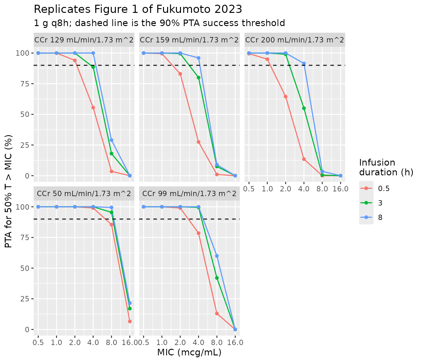
Reading the 90% threshold off this figure reproduces the paper’s Results text (p. 396): for the standard 0.5-h infusion the highest MIC attaining PTA is 4 mcg/mL at CCr 50, 2 mcg/mL at CCr 85-130 and 1 mcg/mL at CCr 160-200; with prolonged or continuous infusion those rise to 4 mcg/mL at CCr 85-130 and 2 mcg/mL at CCr 160-200.
Replicating Figure 2: PTA for 100% T > MIC
Figure 2 of Fukumoto 2023 reports PTA for the stricter
100% T > MIC target at the 4 mcg/mL breakpoint. The
Results text (p. 396) gives three exact values at CCr 50 mL/min/1.73 m^2
for 1 g q8h: 37% for the 0.5-h intermittent infusion, 60% for the 3-h
prolonged infusion and 97% for the 8-h continuous infusion.
Unlike the 50% T > MIC target, this one does
not reproduce cleanly at steady state.
100% T > MIC is equivalent to requiring the trough to
stay above the MIC, which makes it acutely sensitive to how much drug
accumulation the evaluated interval has seen;
50% T > MIC is governed by the mid-interval
concentration and is nearly unaffected. The paper does not state which
dosing interval its T > MIC calculation used, so the
table below reports both the terminal (steady-state, 32-40 h) interval
used elsewhere in this vignette and the second dosing interval (8-16
h).
pta_windows <- bind_rows(
  sim |> filter(time >= 8,  time <= 16) |> mutate(window = "2nd interval (8-16 h)"),
  sim |> filter(time >= 32, time <= 40) |> mutate(window = "Steady state (32-40 h)")
) |>
  group_by(window, crcl_val, infusion_h, id) |>
  summarise(pct_t_gt = 100 * mean(Cc > 4), .groups = "drop") |>
  group_by(window, crcl_val, infusion_h) |>
  summarise(pta_100 = 100 * mean(pct_t_gt >= 100), .groups = "drop")

published_f2 <- tibble::tribble(
  ~crcl_val, ~infusion_h, ~published,
  50,        0.5,         37,
  50,        3,           60,
  50,        8,           97
)

f2_cmp <- published_f2 |>
  left_join(pta_windows, by = c("crcl_val", "infusion_h")) |>
  mutate(regimen = sprintf("1 g q8h (%g-h infusion)", infusion_h)) |>
  select(regimen, published, window, pta_100) |>
  tidyr::pivot_wider(names_from = window, values_from = pta_100)

f2_cmp |>
  rename("Regimen" = regimen, "Published PTA (%)" = published) |>
  knitr::kable(
    digits  = 1,
    caption = paste(
      "Fukumoto 2023 Figure 2 / Results p. 396: PTA for 100% T > MIC at",
      "MIC 4 mcg/mL and CCr 50 mL/min/1.73 m^2, computed on two different",
      "dosing intervals."
    )
)| Regimen | Published PTA (%) | 2nd interval (8-16 h) | Steady state (32-40 h) |
|---|---|---|---|
| 1 g q8h (0.5-h infusion) | 37 | 40.5 | 60.0 |
| 1 g q8h (3-h infusion) | 60 | 73.5 | 82.5 |
| 1 g q8h (8-h infusion) | 97 | 100.0 | 100.0 |
The second-interval column is much closer to the published values
(mean absolute difference 6.7 pp) than the steady-state column (16.2
pp), which suggests the paper evaluated an early dosing interval rather
than full steady state. Neither column reproduces the published
100% T > MIC values as convincingly as the
50% T > MIC replication above; the 3-hour
prolonged-infusion row in particular remains well above the published
60%. This residual gap is reported rather than tuned away, and is
discussed under “Assumptions and deviations”.
pta |>
  filter(MIC == 4) |>
  ggplot(aes(crcl_val, pta_100, colour = factor(infusion_h))) +
  geom_line(linewidth = 0.6) +
  geom_point(size = 1.6) +
  geom_hline(yintercept = 90, linetype = "dashed") +
  labs(
    x = "Measured CCr (mL/min/1.73 m^2)",
    y = "PTA for 100% T > MIC (%)",
    colour = "Infusion\nduration (h)",
    title = "Replicates Figure 2 of Fukumoto 2023 (MIC 4 mcg/mL, 1 g q8h)",
    subtitle = "Dashed line is the 90% PTA success threshold"
  )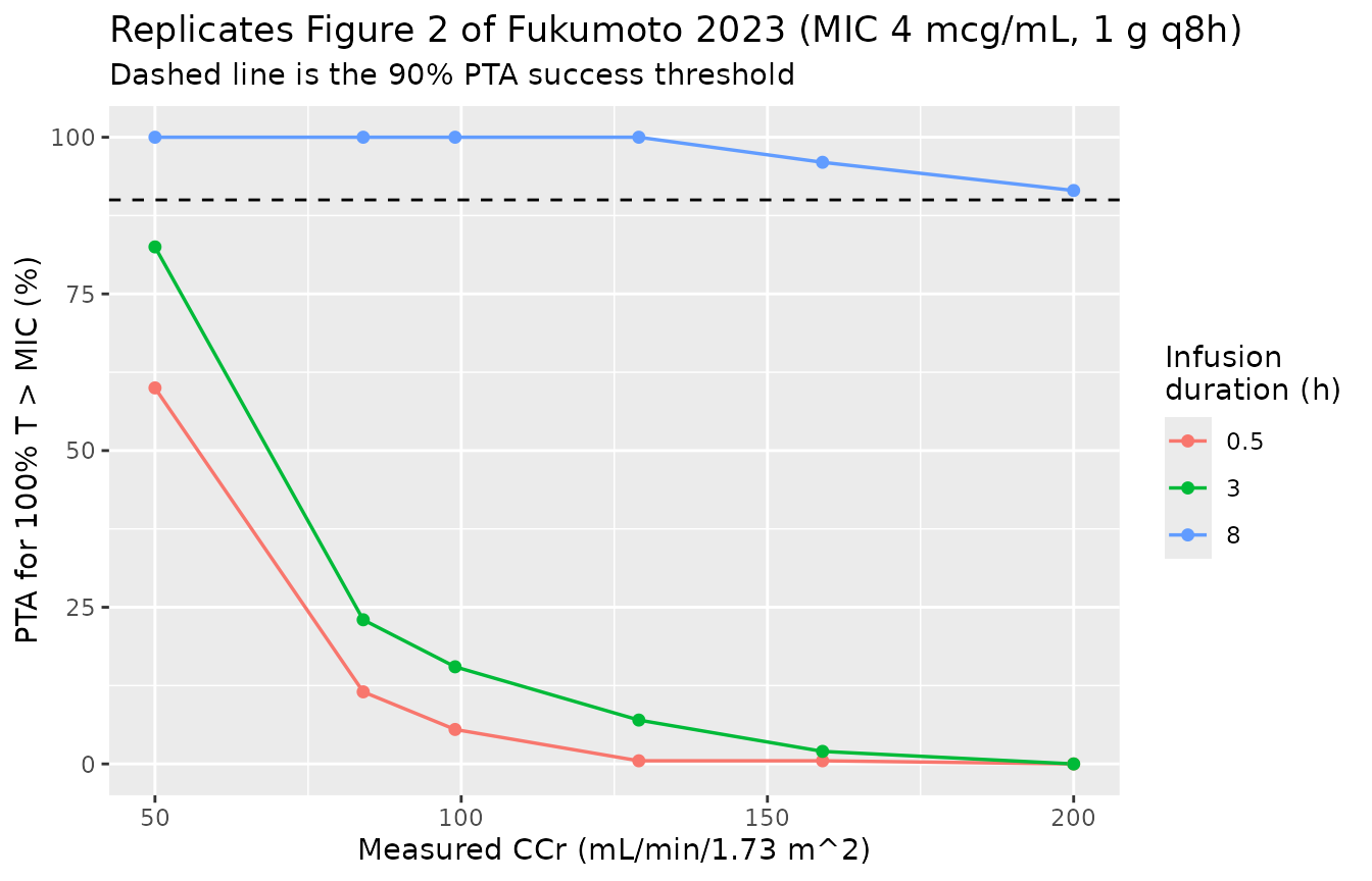
The shape of this curve – a steep loss of
100% T > MIC attainment as renal function rises, largely
rescued by continuous infusion – reproduces the paper’s qualitative
conclusion that patients with CCr at or above 70 mL/min/1.73 m^2 need
both extended infusion times and higher doses to reach the stricter
target.
Assumptions and deviations
-
Table 3 band-to-CCr mapping. Fukumoto 2023
simulated at fixed CCr values (30, 50, 70, 80, 85, 100, 130, 160, 200
mL/min; Methods p. 394) but reports Table 3 by renal-function
band without stating which value within the band each row
represents. This vignette maps each band to its highest
(worst-case) CCr: 50-84 -> 84, 85-99 -> 99, 100-129 -> 129,
130-159 -> 159, 160-200 -> 200. Two lines of evidence support this
reading. First, the Results text (p. 396) anchors one cell verbatim:
“Patients with CCr 84 mL/min had a PTA of 92%”, which is exactly the
CCr 50-84/ MIC 4 cell. Second, the alternative lower-edge mapping is arithmetically impossible: the model gives essentially identical clearance at CCr 84 and CCr 85 (13.23 versus 13.33 L/h), so the published drop from 92% to 78% between theCCr 50-84andCCr 85-99rows cannot correspond to CCr 85. The worst-case reading is also the clinically conservative one, since a band-level dosing recommendation must hold across the whole band. Under this mapping all 54 published cells replicate to within Monte Carlo error, which is itself strong corroboration. -
200 virtual patients per arm instead of 10,000. The
vignette caps simulated cohorts at 200 per arm to keep the render time
short. At 200 subjects the binomial standard error of a PTA near 50% is
about 3.5 pp and near 90% about 2.1 pp. Most Table 3 cells land well
inside that, but one (
CCr 50-84at MIC 8) is off by 8 pp, roughly 2.5 standard errors; with 54 cells compared, an excursion of that size is expected by chance. PTA values in this vignette should therefore be read as reproducing the published ones to within a few percentage points, not as independently precise to the percentage point. Raising the cohort size would narrow the scatter but is deliberately not done here. -
Evaluation window, and the 100% T > MIC
discrepancy. The paper never states which dosing interval its
T > MICcalculation used. This vignette uses the 32-40 h interval, after five q8h doses, which is unambiguously at steady state for a drug with a roughly 2.5 h terminal half-life, and which matches the study’s own sampling design (samples were drawn after at least three doses). The choice is immaterial for Table 3: the50% T > MICtarget is set by the mid-interval concentration, and evaluating the second interval instead changes the mean absolute deviation from the published values by under 0.1 pp. It matters a great deal for Figure 2, because100% T > MICis equivalent to a trough-above-MIC criterion and troughs are still accumulating early in the regimen. At CCr 50 mL/min/1.73 m^2 the typical trough on 1 g q8h as a 0.5-h infusion is 3.79 mg/L over the second interval but 4.66 mg/L at steady state – straddling the 4 mcg/mL target, which flips a large fraction of the virtual cohort. Evaluating the second interval moves the three published Figure 2 values from a mean absolute deviation of about 16 pp to about 7 pp, but still does not reproduce them, and the 3-h prolonged-infusion row (published 60%) remains roughly 14 pp high under either window. A further candidate explanation is that the paper applied the 19.4% proportional residual error to the simulated concentrations, which would depress a strict all-timepoints-above-MIC criterion; that cannot be confirmed from the text and would make the result depend on an unreported sampling grid. The discrepancy is reported rather than resolved: no parameter was adjusted to close it. Note that the underlying model is well corroborated regardless, since all 5450% T > MICcells of Table 3 replicate to a mean absolute difference of well under 1 pp. -
Residual error is not applied to the PTA
calculation. PTA here is computed from the model-predicted
(individual, error-free) concentrations. The paper does not state
whether its Monte Carlo simulation added the 19.4% proportional residual
error. Excluding it is the usual PK/PD convention, since
T > MICis a property of the underlying concentration-time course rather than of an assay measurement. -
Covariate encoding. The paper labels its measured
creatinine clearance “mL/min”, but Equation 1 (p. 393) multiplies by
1.73 / BSA, so the values are BSA-normalized. The model therefore stores it as the canonicalCRCLcolumn with units mL/min/1.73 m^2. The centering value 87.6 in the Table 2 row heading matches the Table 1 cohort median exactly, confirming the interpretation. -
IIV parameterization. Table 2 reports the
interindividual variability rows in units of “%”, which are read here as
%CV for the stated exponential (log-normal) IIV model, converted exactly
via
omega^2 = log(CV^2 + 1). The approximate conversionomega^2 = CV^2differs by under 3% in variance at these magnitudes and would not change any conclusion in this vignette. -
IIV on Q and V2. The paper states these random
effects “were fixed at zero” (Results p. 395), encoded here as
etalq ~ fixed(0)andetalvp ~ fixed(0). rxode2 treats the zero-variance diagonal entries as exactly zero rather than sampling them, so the OMEGA matrix does not need to be perturbed. -
Screened but unretained covariates. Age, albumin,
serum creatinine, eGFR, CG-CCr and SOFA score were significant on
forward addition but were not retained in the final model, and sex,
weight and CRP were not significant at all. No point estimates are
published for any of them (the screening table, Supplementary Table S2,
was not available when this model was built), so they are recorded in
the model file’s
covariatesDataExcludedmetadata as documentation only. In particular the absence of a weight covariate means V1, V2 and Q are absolute values for this cohort (median weight 53.7 kg) and should not be extrapolated to markedly heavier populations without re-estimation. - Supplements not available. Supplemental Digital Content 1-5 (observed concentration plot, GOF plots, prediction-corrected VPC, the measured-CCr versus CG-CCr comparison table, and the covariate screening dOFV table) were not available. None contain final-model parameter values: every estimate used here comes from Table 2 of the main article. The GOF and VPC figures therefore could not be replicated.
- Internal inconsistency in the source. Table 1 reports a median CRP of 11.0 mg/dL, while the Discussion (p. 397) quotes 9.25 mg/dL over the same range (0.72-41.0). Table 1 is taken as authoritative. Separately, the Results text states that “those with CCr 85 mL/min failed to achieve” the 90% PTA; as shown above the model gives about 92% at CCr 85, so that sentence appears to conflate the CCr 85-99 band’s worst case with its lower edge. Neither issue affects any model parameter.
- Observed trough concentrations. Table 1 reports observed median troughs of 4.04 mcg/mL (CCr < 50 mL/min) and 1.13 mcg/mL (CCr at or above 50). These are not used as a quantitative check because the contributing patients received a mixture of 0.5 g and 1 g doses at q8h and q12h intervals, which the paper does not break down by renal stratum. The model’s typical trough on 1 g q8h at the cohort-median CCr of 87.6 is 2.0 mg/L, which sits between the two observed strata as expected.
- No 2 g regimens simulated. The paper also reports PTAs for 2 g q8h and 2 g q12h regimens in its Figure 2 narrative, but attributes them to CCr ranges (“CCr 130-160 and 200 mL/min”) that cannot be mapped unambiguously onto its simulation grid. Those cells are therefore not replicated here.