Doxorubicin + sorafenib combination tumor growth inhibition in mice (Choi 2021)
Source:vignettes/articles/Choi_2021_doxorubicin_sorafenib_mouse.Rmd
Choi_2021_doxorubicin_sorafenib_mouse.RmdModels and source
Choi 2021 builds integrated PK-PD models for doxorubicin (Dox, IV) and sorafenib (Sor, oral) in mice bearing orthotopic human 143B osteosarcoma xenografts, then compares the conventional Koch 2009 combination model (in which an interaction factor has to be assigned to one drug, giving two alternatives, C1 and C2) with a new model D that weights each drug’s kill term by a contribution factor. All five fitted models are distributed:
| File | Choi 2021 model | Estimated in the tumor fit |
|---|---|---|
Choi_2021_doxorubicin_mouse |
Model A: Dox monotherapy (Table 1 Dox iv, Table 2 Dox) | w0, k1, k2 |
Choi_2021_sorafenib_mouse |
Model B: Sor monotherapy (Table 1 Sor iv + p.o., Table 2 Sor) | w0, k1, k2 |
Choi_2021_doxorubicin_sorafenib_mouse |
Model D: contribution factors a (Dox) and b (Sor) (Table 3) | w0, k1’, a, b |
Choi_2021_doxorubicin_sorafenib_c1_mouse |
Model C1: interaction factor on Dox (Table 3) | w0, k1’, C_Dox |
Choi_2021_doxorubicin_sorafenib_c2_mouse |
Model C2: interaction factor on Sor (Table 3) | w0, k1’, C_Sor |
nms <- c(
  dox = "Choi_2021_doxorubicin_mouse",
  sor = "Choi_2021_sorafenib_mouse",
  D = "Choi_2021_doxorubicin_sorafenib_mouse",
  C1 = "Choi_2021_doxorubicin_sorafenib_c1_mouse",
  C2 = "Choi_2021_doxorubicin_sorafenib_c2_mouse"
)
ui <- lapply(nms, function(n) rxode2::rxode(readModelDb(n)))
# No model carries inter-animal variability (Choi 2021 fitted typical values in
# SimBiology); zeroRe() only removes the residual error for typical-value runs.
tv <- lapply(ui, function(u) suppressWarnings(rxode2::zeroRe(u)))
stopifnot(all(vapply(ui, function(u) is.null(u$linCmt), logical(1))))- Citation: Choi YH, Zhang C, Liu Z, Tu MJ, Yu AX, Yu AM. A Novel Integrated Pharmacokinetic-Pharmacodynamic Model to Evaluate Combination Therapy and Determine In Vivo Synergism. J Pharmacol Exp Ther. 2021;377(3):305-315. doi:10.1124/jpet.121.000584. Tumor-growth data and dosing regimen from Jian C, Tu MJ, Ho PY, et al. Oncotarget. 2017;8(19):30742-30755. doi:10.18632/oncotarget.16372.
- Article (open access): https://doi.org/10.1124/jpet.121.000584
- Supplement: Supplementary Methods (equations S1-S3 for models C1 and
C2), Figures S1-S3 and Table S1, distributed as
584SupplData.pdfon the journal site. The “MATLAB files available online” were not deposited with it. - Tumor data and dosing regimen: Jian 2017, https://doi.org/10.18632/oncotarget.16372
Crossref lists no correction or erratum for this article (checked 2026-09-28).
Population
PK was measured in tumor-free male athymic nude mice (about 30 g, 7 weeks old, n = 6 per arm): Dox 0.06 mg IV, Sor 0.02 mg IV and Sor 0.2 mg by oral gavage. The tumor-growth data come from Jian 2017: female CB17 SCID mice with intratibial 143B-GFP-Luc osteosarcoma xenografts, n = 7 per group, given vehicle, Dox (12 ug IV every other day x4, then 10 ug x4), Sor (200 ug oral on 7 days, then every other day x4) or both. Five of the seven combination mice were used to fit models C1, C2 and D and the remaining two to verify model D (Choi 2021 Methods).
pop <- ui$D$population
tibble::tibble(Field = names(pop), Value = vapply(pop, function(x) paste(x, collapse = "; "), character(1))) |>
knitr::kable()| Field | Value |
|---|---|
| species | mouse (PK: male athymic nude Foxn1nu; tumor growth: female CB17 SCID with orthotopic 143B osteosarcoma xenograft) |
| n_subjects | 23 |
| n_studies | 2 |
| age_range | 7 weeks at purchase (PK mice) |
| weight_range | approximately 30 g (PK mice) |
| sex_female_pct | NA |
| race_ethnicity | NA |
| disease_state | PK: tumor-free mice. PD: orthotopic (intratibial) human 143B osteosarcoma cell-line-derived xenograft. |
| dose_range | PD: doxorubicin 12 ug/mouse IV every other day x4 then 10 ug/mouse IV every other day x4, plus sorafenib 200 ug/mouse oral gavage on 7 days of cycle 1 then every other day x4 in cycle 2, per Jian 2017. |
| regions | University of California Davis, USA (preclinical) |
| notes | PK: n = 6 male athymic nude mice per arm (doxorubicin IV, sorafenib IV, sorafenib oral; Choi 2021 Table 1). PD: 5 of the 7 combination- treated tumor-bearing mice from Jian 2017 were randomly chosen for model development and the remaining 2 used for verification (Choi 2021 Methods; Table 3). Only w0, k1’ and the contribution factors a and b were estimated; the PK, the natural-growth rates and each drug’s potency k2 were held at their earlier estimates. |
Source trace
Every ini() value carries an in-file comment naming its
source. Summary:
| Parameter (files) | Value | Source |
|---|---|---|
Dox lvc, lvp, lk12,
lk21, lkel (A; _dox in
C1/C2/D) |
0.0764 L, 3.52 L, 5.86, 0.127, 1.24 1/h | Table 1, Dox (iv) |
Sor lvc, lvp, lk12,
lk21, lkel (B; _sorafenib in
C1/C2/D) |
0.0112 L, 0.0120 L, 0.663, 0.620, 0.344 1/h | Table 1, Sor (iv) |
Sor lka
|
0.640 1/h | Table 1, Sor (p.o.) |
ltumorExpGrowth (L0), ltumorLinGrowth
(L1), all files, fixed |
0.107 1/day, 0.148 cm^3/day | Table 2, Control; Table 2/3 footnote a |
Dox lrbase_tumor, ldamageTransit,
ldrugSlope
|
0.0386 cm^3, 0.130 1/day, 13.8 L/mg/day | Table 2, Dox |
Sor lrbase_tumor, ldamageTransit,
ldrugSlope
|
0.0415 cm^3, 17.0 1/day, 0.0267 L/mg/day | Table 2, Sor |
D lrbase_tumor, ldamageTransit,
lcontrib_dox, lcontrib_sorafenib
|
0.0422, 0.832, 0.644, 1.62 | Table 3, Model D |
C1 lrbase_tumor, ldamageTransit,
linteract_dox
|
0.0382, 1.00, 2.78 | Table 3, Model C1 |
C2 lrbase_tumor, ldamageTransit,
linteract_sorafenib
|
0.0405, 0.451, 1.56 | Table 3, Model C2 |
expSd* residual SDs |
sqrt(MSE) | Tables 1-3 MSE rows (see Assumptions) |
| Two-compartment PK ODEs | – | Equations 1-5 |
| Koch 2009 growth + three-stage transit (A, B) | – | Equations 8-14 |
Model D kill term a*k2A*C_A + b*k2B*C_B
|
– | Equations 15-21, Figure 1D |
| Models C1 / C2 kill terms | – | Supplementary equations S1-S3, Figure 1C |
Single-dose PK (Figure 2A)
Model time is days; the PK rate constants are printed in 1/h and
multiplied by 24 inside model(). The monotherapy files
declare two endpoints (Cc and tumor_vol), so
every observation row nominates one through dvid; both
outputs are returned regardless.
pk_events <- function(amt, cmt, hours, treatment) {
  dplyr::bind_rows(
    data.frame(time = 0, amt = amt, cmt = cmt, evid = 1L, dvid = NA_integer_),
    data.frame(time = hours / 24, amt = NA_real_, cmt = NA_character_, evid = 0L, dvid = 1L)
  ) |>
    dplyr::mutate(id = 1L, treatment = treatment, .before = 1)
}
pk_solve <- function(mod, ev) {
  out <- as.data.frame(rxode2::rxSolve(mod, ev, returnType = "data.frame", rtol = 1e-10, atol = 1e-12))
  out$treatment <- ev$treatment[1]
  out
}
# Log-spaced early grid: Dox leaves the central compartment with a half-life
# of about 5 minutes (k12 + ke = 7.1 1/h).
hours <- sort(unique(c(0, 10^seq(-3, log10(400), length.out = 400))))
pk <- dplyr::bind_rows(
  pk_solve(tv$dox, pk_events(0.06, "central", hours, "Dox 0.06 mg IV")),
  pk_solve(tv$sor, pk_events(0.02, "central", hours, "Sor 0.02 mg IV")),
  pk_solve(tv$sor, pk_events(0.2, "depot", hours, "Sor 0.2 mg p.o."))
) |>
  dplyr::mutate(id = 1L, hours = time * 24)
ggplot(dplyr::filter(pk, hours > 0, hours <= 48), aes(hours, Cc)) +
  geom_line(colour = "steelblue") +
  facet_wrap(~treatment, scales = "free_y") +
  scale_y_log10() +
  labs(x = "Time (h)", y = "Plasma concentration (mg/L)")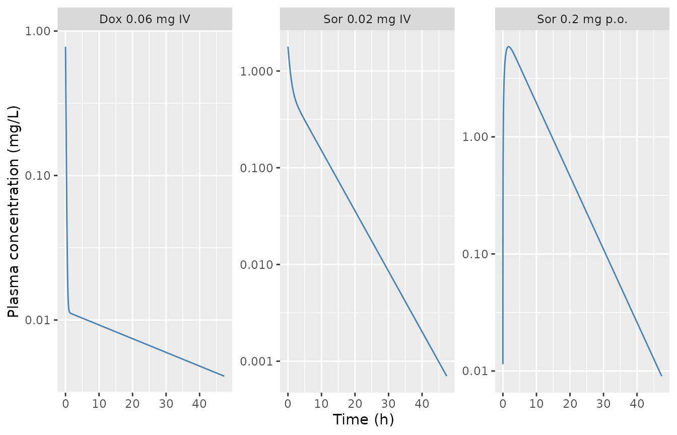
Replicates Figure 2A of Choi 2021 (typical-value predictions).
The curves match Figure 2A: Dox falls from about 0.8 mg/L to a 0.01 mg/L plateau within 3 h and is 0.007 mg/L at 24 h; oral Sor peaks near 6 mg/L at 2 h and is about 0.01 mg/L at 48 h.
PKNCA
Choi 2021 reports no NCA table, so PKNCA is checked against the
closed form of a linear two-compartment model,
AUC(0-inf) = Dose / (ke * Vc) (oral F = 1).
conc <- pk |>
  dplyr::filter(!is.na(Cc)) |>
  dplyr::select(id, treatment, time = hours, Cc) |>
  dplyr::mutate(Cc = pmax(Cc, 0))
doses <- data.frame(
  id = 1L, time = 0,
  treatment = c("Dox 0.06 mg IV", "Sor 0.02 mg IV", "Sor 0.2 mg p.o."),
  amt = c(0.06, 0.02, 0.2),
  route = c("intravascular", "intravascular", "extravascular")
)
o_conc <- PKNCA::PKNCAconc(conc, Cc ~ time | treatment + id, concu = "mg/L", timeu = "h")
o_dose <- PKNCA::PKNCAdose(doses, amt ~ time | treatment + id, route = "route", doseu = "mg")
o_data <- PKNCA::PKNCAdata(o_conc, o_dose,
  intervals = data.frame(start = 0, end = Inf, cmax = TRUE, tmax = TRUE, aucinf.obs = TRUE, half.life = TRUE)
)
nca <- as.data.frame(PKNCA::pk.nca(o_data))
nca_wide <- nca |>
  dplyr::select(treatment, PPTESTCD, PPORRES) |>
  tidyr::pivot_wider(names_from = PPTESTCD, values_from = PPORRES)
analytic <- data.frame(
  treatment = doses$treatment,
  auc_analytic = doses$amt / c(1.24 * 0.0764, 0.344 * 0.0112, 0.344 * 0.0112)
)
nca_tab <- dplyr::left_join(nca_wide, analytic, by = "treatment") |>
  dplyr::mutate(pct_diff = 100 * (aucinf.obs / auc_analytic - 1))
nca_tab |>
  dplyr::transmute(
    Treatment = treatment,
    "Cmax (mg/L)" = signif(cmax, 3),
    "Tmax (h)" = signif(tmax, 3),
    "t1/2 (h)" = signif(half.life, 3),
    "AUC0-inf PKNCA (mg*h/L)" = signif(aucinf.obs, 4),
    "Dose/(ke*Vc) (mg*h/L)" = signif(auc_analytic, 4),
    "Difference (%)" = round(pct_diff, 2)
  ) |>
knitr::kable()| Treatment | Cmax (mg/L) | Tmax (h) | t1/2 (h) | AUC0-inf PKNCA (mg*h/L) | Dose/(keVc) (mgh/L) | Difference (%) |
|---|---|---|---|---|---|---|
| Dox 0.06 mg IV | 0.785 | 0.0 | 31.70 | 0.6333 | 0.6333 | 0 |
| Sor 0.02 mg IV | 1.790 | 0.0 | 4.80 | 5.1910 | 5.1910 | 0 |
| Sor 0.2 mg p.o. | 5.900 | 1.7 | 4.82 | 51.9100 | 51.9100 | 0 |
Multiple-dose PK in the tumor study (Supplementary Figure S1)
Jian 2017 inoculated the tumors on day 0, measured tumor volume on days 9, 14, 21, 28 and 34, and started treatment on day 11. Choi 2021 Figures 2B and 3 put the first tumor measurement at time 0, so model day = Jian day - 9. The dose times used below are exactly those of Supplementary Figure S1: Dox on days 2, 4, 6, 8 (12 ug) and 15, 17, 19, 21 (10 ug); Sor 0.2 mg on days 2-6, 8, 9 and 15, 17, 19, 21.
dox_times <- c(2, 4, 6, 8, 15, 17, 19, 21)
dox_amts <- c(rep(0.012, 4), rep(0.010, 4))
sor_times <- c(2, 3, 4, 5, 6, 8, 9, 15, 17, 19, 21)
sor_amt <- 0.2
grid <- seq(0, 30, by = 0.02)

# Monotherapy files: 2 endpoints, observation rows nominate tumor_vol by dvid = 2.
mono_events <- function(dose_cmt = NULL, times = NULL, amts = NULL) {
  obs <- data.frame(time = grid, amt = NA_real_, cmt = NA_character_, evid = 0L, dvid = 2L)
  dose <- if (is.null(dose_cmt)) NULL else
    data.frame(time = times, amt = amts, cmt = dose_cmt, evid = 1L, dvid = NA_integer_)
  dplyr::bind_rows(dose, obs) |> dplyr::arrange(time, -evid) |> dplyr::mutate(id = 1L, .before = 1)
}
solve_df <- function(mod, ev, params = NULL) {
  out <- as.data.frame(rxode2::rxSolve(mod, ev, params = params, returnType = "data.frame"))
  if (is.null(out$id)) out$id <- 1L
  out
}
md_dox <- solve_df(tv$dox, mono_events("central", dox_times, dox_amts))
md_sor <- solve_df(tv$sor, mono_events("depot", sor_times, rep(sor_amt, length(sor_times))))
dplyr::bind_rows(
  dplyr::mutate(md_dox, drug = "Dox"),
  dplyr::mutate(md_sor, drug = "Sor")
) |>
  dplyr::filter(Cc > 1e-10) |>
  ggplot(aes(time, Cc)) +
  geom_line(colour = "steelblue") +
  facet_wrap(~drug, scales = "free_y") +
  scale_y_log10() +
  labs(x = "Time (day)", y = "Plasma concentration (mg/L)")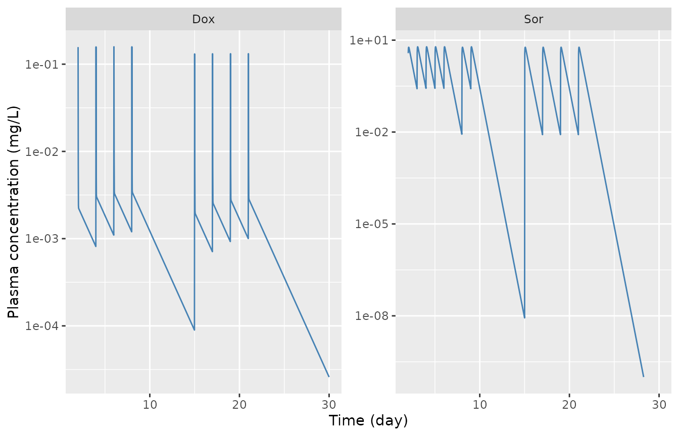
Replicates Supplementary Figure S1 of Choi 2021.
Monotherapy tumor growth (Figure 2B)
The vehicle arm is the natural-growth model alone: the Dox file with no dose and the control-fit initial volume w0 = 0.0412 cm^3 (Table 2, Control). The figure values below were digitized by the maintainers from the model curves in Figure 2B.
ctrl <- solve_df(tv$dox, mono_events(), params = c(lrbase_tumor = log(0.0412)))
mono <- dplyr::bind_rows(
  dplyr::mutate(ctrl, arm = "Control"),
  dplyr::mutate(md_dox, arm = "Dox"),
  dplyr::mutate(md_sor, arm = "Sor")
)
vol_at <- function(df, t) approx(df$time, df$tumor_vol, t)$y
fig2b <- tibble::tribble(
  ~arm, ~day, ~figure,
  "Control", 12, 0.37, "Control", 19, 0.80, "Control", 25, 1.33, "Control", 30, 1.84,
  "Dox", 12, 0.27, "Dox", 19, 0.57, "Dox", 25, 0.93, "Dox", 30, 1.26,
  "Sor", 12, 0.26, "Sor", 19, 0.60, "Sor", 25, 0.98, "Sor", 30, 1.42
)
fig2b$model <- mapply(function(a, d) vol_at(dplyr::filter(mono, arm == a), d), fig2b$arm, fig2b$day)
fig2b <- dplyr::mutate(fig2b, pct_diff = 100 * (model / figure - 1))
fig2b |>
  dplyr::mutate(model = round(model, 3), pct_diff = round(pct_diff, 1)) |>
  dplyr::rename("Arm" = arm, "Day" = day, "Figure 2B (cm^3)" = figure, "Model (cm^3)" = model, "Difference (%)" = pct_diff) |>
knitr::kable()| Arm | Day | Figure 2B (cm^3) | Model (cm^3) | Difference (%) |
|---|---|---|---|---|
| Control | 12 | 0.37 | 0.346 | -6.5 |
| Control | 19 | 0.80 | 0.801 | 0.1 |
| Control | 25 | 1.33 | 1.335 | 0.4 |
| Control | 30 | 1.84 | 1.850 | 0.5 |
| Dox | 12 | 0.27 | 0.257 | -4.7 |
| Dox | 19 | 0.57 | 0.563 | -1.2 |
| Dox | 25 | 0.93 | 0.905 | -2.7 |
| Dox | 30 | 1.26 | 1.260 | 0.0 |
| Sor | 12 | 0.26 | 0.248 | -4.5 |
| Sor | 19 | 0.60 | 0.573 | -4.5 |
| Sor | 25 | 0.98 | 0.953 | -2.7 |
| Sor | 30 | 1.42 | 1.418 | -0.1 |
# Deterministic typical-value curves vs a digitized figure (reading error
# about 0.03 cm^3): a wrong L0/L1 form, k2 unit or dose moves these by tens of %.
stopifnot(all(abs(fig2b$pct_diff) < 10))
ggplot(mono, aes(time, tumor_vol, colour = arm)) +
  geom_line() +
  geom_point(data = fig2b, aes(day, figure, colour = arm), shape = 4, size = 3) +
  labs(x = "Time (day)", y = "Tumor volume (cm^3)", colour = NULL,
       caption = "Lines: model; crosses: Figure 2B curve digitized.")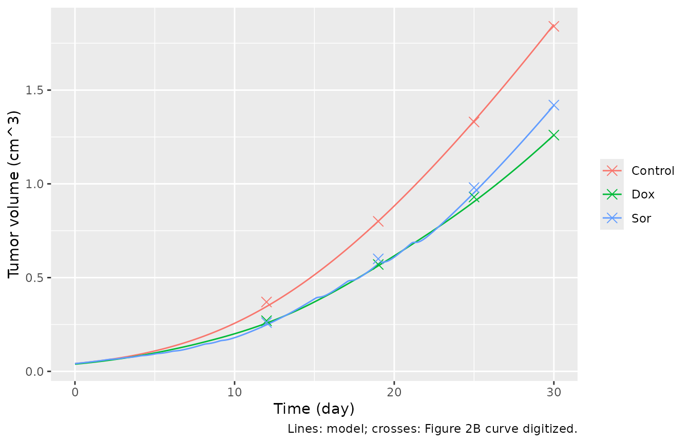
Replicates the model curves of Figure 2B of Choi 2021.
Time efficacy index (Discussion, equation 22)
Choi 2021 gives TEI = k2 * AUC / L0 and reports TEI of
4.67 days (Dox) and 7.20 days (Sor) “at tumor volume of 0.85 cm^3”,
i.e. read from the growth curves. The table gives the equation-22 value
from the total simulated AUC and the horizontal delay between the
treated and control model curves at 0.85 cm^3.
auc_total <- c(
  Dox = sum(dox_amts) / (1.24 * 24 * 0.0764),
  Sor = length(sor_times) * sor_amt / (0.344 * 24 * 0.0112)
)
t_at <- function(df, v) approx(df$tumor_vol, df$time, v)$y
tei <- data.frame(
  drug = c("Dox", "Sor"),
  eq22 = unname(c(13.8, 0.0267) * auc_total / 0.107),
  curve = c(t_at(md_dox, 0.85), t_at(md_sor, 0.85)) - t_at(ctrl, 0.85),
  paper = c(4.67, 7.20)
)
tei |>
  dplyr::mutate(dplyr::across(c(eq22, curve), function(x) round(x, 2))) |>
  dplyr::rename("Drug" = drug, "Eq. 22 (day)" = eq22, "Curve delay at 0.85 cm^3 (day)" = curve, "Choi 2021 (day)" = paper) |>
knitr::kable()| Drug | Eq. 22 (day) | Curve delay at 0.85 cm^3 (day) | Choi 2021 (day) |
|---|---|---|---|
| Dox | 4.99 | 4.51 | 4.67 |
| Sor | 5.94 | 4.16 | 7.20 |
Both Dox values are within 7% of the published 4.67 days. For Sor both model-based values (5.9 and 4.2 days) are below the published 7.20 days. The paper does not say whether its TEI values were read from the observed data or from the model curves, so the Sor difference cannot be attributed; it is reported here, not asserted.
Combination therapy (Figure 3)
The combination files declare three endpoints (Cc_dox,
Cc_sorafenib, tumor_vol). With three endpoints
rxode2 requires the observation row to name the endpoint itself, so
these rows use cmt = "tumor_vol"; the guard below confirms
that the doses still land in the named ODE states.
combo_events <- function(dox_scale = 1, sor_scale = 1) {
  dplyr::bind_rows(
    data.frame(time = dox_times, amt = dox_amts * dox_scale, cmt = "central_dox", evid = 1L),
    data.frame(time = sor_times, amt = sor_amt * sor_scale, cmt = "depot_sorafenib", evid = 1L),
    data.frame(time = grid, amt = NA_real_, cmt = "tumor_vol", evid = 0L)
  ) |>
    dplyr::arrange(time, -evid) |>
    dplyr::mutate(id = 1L, .before = 1)
}
guard <- solve_df(tv$D, combo_events())
stopifnot(
  all(ui$D$state %in% names(guard)),
  all(c("Cc_dox", "Cc_sorafenib", "tumor_vol") %in% names(guard)),
  # First Dox dose on day 2: Cc_dox peaks at 0.012 / 0.0764 = 0.157 mg/L, and
  # sorafenib reaches its multiple-dose peak range of Figure S1B (several mg/L).
  abs(max(guard$Cc_dox) / 0.157 - 1) < 0.05,
  max(guard$Cc_sorafenib) > 3
)
Internal consistency: model D contains model A
With b = 0, a = 1, k1' = 0.130
and w0 = 0.0386 model D is algebraically the Dox
monotherapy model, so the two files must give the same curve.
nested <- solve_df(tv$D, combo_events(sor_scale = 0), params = c(
  lcontrib_dox = 0, lcontrib_sorafenib = log(1e-12),
  ldamageTransit = log(0.130), lrbase_tumor = log(0.0386)
))
nested_diff <- max(abs(vol_at(nested, c(5, 12, 19, 25, 30)) / vol_at(md_dox, c(5, 12, 19, 25, 30)) - 1))
nested_diff
#> [1] 5.432448e-07
# Same ODE system integrated by LSODA at default tolerance: agreement ~1e-6.
stopifnot(nested_diff < 1e-4)
Reproduction of Figure 3
combo <- dplyr::bind_rows(lapply(c("D", "C1", "C2"), function(m) {
  dplyr::bind_rows(
    dplyr::mutate(solve_df(tv[[m]], combo_events()), model = m, dox_exposure = "As published (1x)"),
    dplyr::mutate(solve_df(tv[[m]], combo_events(dox_scale = 0.37)), model = m, dox_exposure = "Diagnostic (0.37x)")
  )
}))
fig3 <- tibble::tribble(
  ~model, ~day, ~figure,
  "C1", 12, 0.17, "C1", 19, 0.40, "C1", 25, 0.60, "C1", 30, 0.92,
  "C2", 12, 0.15, "C2", 19, 0.35, "C2", 25, 0.53, "C2", 30, 0.81,
  "D", 12, 0.17, "D", 19, 0.39, "D", 25, 0.60, "D", 30, 0.93
)
pick <- function(m, d, e) vol_at(dplyr::filter(combo, model == m, dox_exposure == e), d)
fig3$as_published <- mapply(pick, fig3$model, fig3$day, "As published (1x)")
fig3$diagnostic <- mapply(pick, fig3$model, fig3$day, "Diagnostic (0.37x)")
fig3 |>
  dplyr::mutate(dplyr::across(c(as_published, diagnostic), function(x) round(x, 3))) |>
  dplyr::rename(
    "Model" = model, "Day" = day, "Figure 3 (cm^3)" = figure,
    "Published parameters + regimen (cm^3)" = as_published,
    "Same, Dox exposure x 0.37 (cm^3)" = diagnostic
  ) |>
knitr::kable()| Model | Day | Figure 3 (cm^3) | Published parameters + regimen (cm^3) | Same, Dox exposure x 0.37 (cm^3) |
|---|---|---|---|---|
| C1 | 12 | 0.17 | 0.092 | 0.157 |
| C1 | 19 | 0.40 | 0.193 | 0.366 |
| C1 | 25 | 0.60 | 0.247 | 0.555 |
| C1 | 30 | 0.92 | 0.442 | 0.889 |
| C2 | 12 | 0.15 | 0.134 | 0.159 |
| C2 | 19 | 0.35 | 0.255 | 0.330 |
| C2 | 25 | 0.53 | 0.375 | 0.515 |
| C2 | 30 | 0.81 | 0.589 | 0.794 |
| D | 12 | 0.17 | 0.144 | 0.162 |
| D | 19 | 0.39 | 0.324 | 0.374 |
| D | 25 | 0.60 | 0.484 | 0.578 |
| D | 30 | 0.93 | 0.791 | 0.923 |
ggplot(combo, aes(time, tumor_vol, colour = dox_exposure)) +
  geom_line() +
  geom_point(data = fig3, aes(day, figure), inherit.aes = FALSE, shape = 4, size = 3) +
  facet_wrap(~model) +
  labs(x = "Time (day)", y = "Tumor volume (cm^3)", colour = NULL) +
  theme(legend.position = "bottom")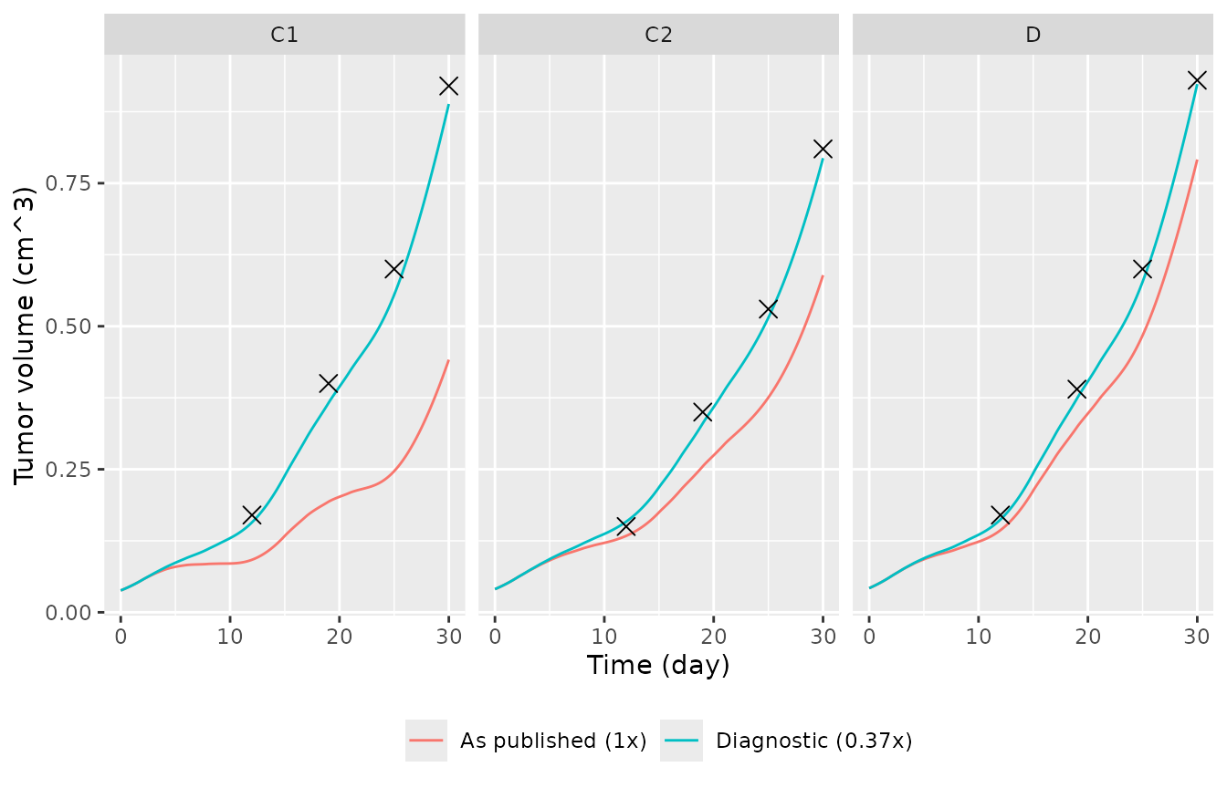
Figure 3 of Choi 2021 (crosses, digitized) against the packaged combination models.
The published combination figures do not follow from the published parameters and regimen. With Table 3 parameters, the Table 1 PK and the Figure S1 dose schedule, all three combination models predict more tumor suppression than Figure 3 shows (at day 30: D 0.79 vs 0.93 cm^3, C2 0.59 vs 0.81, C1 0.44 vs 0.92). The monotherapy arms, which share the same Dox and Sor PK code and the same dose schedule, reproduce Figure 2B and Figure S1 within a few percent (above), so the transcription of the shared parts is not the cause.
A single change reproduces every combination curve: scaling the Dox exposure in the combination runs by about 0.37. That factor was found by eye against Figure 3 and then checked, without further adjustment, against the 12 dose combinations of Figure 4B below. It is consistent with the three conventional and new models all fitting the same five mice about equally well (Table 3 MSE 0.120-0.130): C1 multiplies the Dox term by 2.78 and C2 the Sor term by 1.56, and both can describe the same data only if the Dox kill term is about one third of the Sor term. Neither the paper nor its supplement states a Dox input for the combination runs that differs from Figure S1, and the MATLAB files were not deposited, so the origin of the factor cannot be traced. The packaged files keep the published values; the 0.37 factor is a diagnostic used only in this article and is not part of any model.
# As published, every combination model sits below Figure 3 at days 19-30
# (the documented discrepancy; if this ever fails, re-check the files and this
# section).
stopifnot(all(fig3$as_published[fig3$day >= 19] < fig3$figure[fig3$day >= 19]))
# The diagnostic reproduces Figure 3 within the digitizing tolerance.
stopifnot(all(abs(fig3$diagnostic / fig3$figure - 1) < 0.10))
Dose-combination predictions (Figure 4B)
fig4b <- tibble::tribble(
  ~dox, ~sor, ~figure,
  1, 0.5, 1.29, 1, 1, 0.93, 1, 1.5, 0.65, 1, 2, 0.43,
  0.5, 1, 0.96, 1.5, 1, 0.90, 2, 1, 0.86,
  0.5, 0.5, 1.34, 0.5, 2, 0.45, 2, 0.5, 1.20, 2, 2, 0.39
)
day30 <- function(m, d, s) vol_at(solve_df(tv[[m]], combo_events(dox_scale = d, sor_scale = s)), 30)
fig4b$as_published <- mapply(function(d, s) day30("D", d, s), fig4b$dox, fig4b$sor)
fig4b$diagnostic <- mapply(function(d, s) day30("D", 0.37 * d, s), fig4b$dox, fig4b$sor)
fig4b |>
  dplyr::mutate(
    label = paste0(dox, "Dox + ", sor, "Sor"),
    dplyr::across(c(as_published, diagnostic), function(x) round(x, 3))
  ) |>
  dplyr::select(label, figure, as_published, diagnostic) |>
  dplyr::rename(
    "Combination (fold of experimental dose)" = label, "Figure 4B, day 30 (cm^3)" = figure,
    "Published parameters (cm^3)" = as_published, "Dox exposure x 0.37 (cm^3)" = diagnostic
  ) |>
knitr::kable()| Combination (fold of experimental dose) | Figure 4B, day 30 (cm^3) | Published parameters (cm^3) | Dox exposure x 0.37 (cm^3) |
|---|---|---|---|
| 1Dox + 0.5Sor | 1.29 | 1.110 | 1.277 |
| 1Dox + 1Sor | 0.93 | 0.791 | 0.923 |
| 1Dox + 1.5Sor | 0.65 | 0.538 | 0.641 |
| 1Dox + 2Sor | 0.43 | 0.342 | 0.420 |
| 0.5Dox + 1Sor | 0.96 | 0.895 | 0.965 |
| 1.5Dox + 1Sor | 0.90 | 0.697 | 0.883 |
| 2Dox + 1Sor | 0.86 | 0.610 | 0.844 |
| 0.5Dox + 0.5Sor | 1.34 | 1.241 | 1.330 |
| 0.5Dox + 2Sor | 0.45 | 0.403 | 0.444 |
| 2Dox + 0.5Sor | 1.20 | 0.879 | 1.177 |
| 2Dox + 2Sor | 0.39 | 0.241 | 0.373 |
Both versions agree with the paper’s qualitative conclusion that, under model D, tumor growth is far more sensitive to the Sor dose than to the Dox dose. As published, however, model D is noticeably more Dox-sensitive than Figure 4B (2Dox + Sor gives 0.61 cm^3 instead of 0.86).
Assumptions and deviations
-
Time unit. Model time is days (the tumor time
scale). The PK rate constants are kept in
ini()as printed (1/h) and multiplied by 24 inmodel(); all doses are in mg and concentrations in mg/L. -
Residual error. Choi 2021 used an exponential error
model but does not print its magnitude. Each
expSdissqrt(MSE)of the corresponding fit. The tumor-fit MSEs equal SSE / (n - p) exactly (for example 4.72 / 0.148 = 32 = 35 - 3 for Dox; 2.72 / 0.130 = 21 = 25 - 4 for model D), and the residual plots of Figures 2B and 3 are on the log scale (residuals of +/-0.5 at a 0.04 cm^3 tumor), so the MSE is the log-scale residual variance. The Sor concentration SD uses the oral-arm MSE (0.337; IV arm 0.0741). The combination files carry the monotherapy PK SDs as fixed values. - No inter-animal variability. None was estimated (SimBiology typical-value fit); the %CV values in Tables 1-3 are estimate precision.
- Sorafenib bioavailability. Only ka was estimated from the oral data with the IV disposition fixed, so F = 1 is implicit.
-
Fixed parameters. L0 and L1 are
fixed()in every file (Table 2 and 3 footnotes). In the combination files the PK and both potencies k2 arefixed()because they were carried from the monotherapy fits. In the monotherapy files the PK parameters are left estimable because they were estimated from the PK data in the first step of the sequential fit. -
Control arm. The vehicle fit (w0 = 0.0412 cm^3) has
no drug and is not a separate file; it is the Dox file with no dose and
lrbase_tumorset to log(0.0412). - Dosing times. Taken from Jian 2017 Figure 3A shifted by 9 days, which matches the dose times drawn in Choi 2021 Figure S1.
- Combination-figure discrepancy. See the Figure 3 section: as published, models C1, C2 and D predict more suppression than Figures 3 and 4. The packaged values are not adjusted.
- Not extracted. Combination-index (CI) values, computed with CompuSyn, are not a model output. Supplementary Table S1 gives fits of models C1, C2 and D to five hypothetical tumor-growth profiles, which are illustrations rather than models of observed data.
- Mixed animal strains. As in the paper, PK from male athymic nude mice drives tumor growth in female SCID mice; Choi 2021 notes this as a limitation.