Diao_2016_daclizumab_treg • nlmixr2lib

library(nlmixr2lib)
library(rxode2)
#> rxode2 5.0.2 using 2 threads (see ?getRxThreads)
#>   no cache: create with `rxCreateCache()`
library(dplyr)
#> 
#> Attaching package: 'dplyr'
#> The following objects are masked from 'package:stats':
#> 
#>     filter, lag
#> The following objects are masked from 'package:base':
#> 
#>     intersect, setdiff, setequal, union
library(tidyr)
library(ggplot2)
library(PKNCA)
#> 
#> Attaching package: 'PKNCA'
#> The following object is masked from 'package:stats':
#> 
#>     filter

Daclizumab HYP regulatory T cell (Treg) reduction PK/PD model

CD25 is constitutively expressed at high levels on regulatory T cells (Treg, defined here as CD4+ CD127low/- Foxp3+). Daclizumab high-yield process (HYP) reduces circulating Treg counts during treatment despite maintaining clinical efficacy in RRMS. Diao et al. (2016) characterized the reduction with an algebraic sigmoidal Emax model linking daclizumab HYP serum concentration directly to Treg percentage of CD4+ T cells; adding a delay / effect compartment did not improve fit (Diao 2016 Discussion).

The PK backbone is inherited from Othman 2014 (two-compartment first-order SC absorption with lag, allometric weight scaling); see the companion Othman_2014_daclizumab vignette for the PK details.

Citation: Diao L, Hang Y, Othman AA, et al. Br J Clin Pharmacol. 2016;82(5):1333-1342.
Article: https://doi.org/10.1111/bcp.13051
PMID: 27333593

Population

The pooled PK/PD analysis included 1353 RRMS subjects with 8742 Treg records from four daclizumab HYP clinical studies (Diao 2016 Table 2):

Study	Subjects	Treg records
205MS201 / SELECT and 205MS202 / SELECTION	545	4835
205MS302 / OBSERVE	106	891
205MS301 / DECIDE	702	3016

The typical baseline Treg percentage among CD4+ T cells is 12.1% (Diao 2016 Table 5).

Source trace

Equation / parameter	Value	Source
PK backbone (`lka`, `lcl`, `lvc`, `lvp`, `lq`, `lfdepot`, `lalag`, `allo_*`, `e_dose_50mg_f`, PK IIV, `CcpropSd`, `CcaddSd`)	Othman 2014 Table 2 values	inherited from `Othman_2014_daclizumab.R`
`ltregE0` (typical baseline Treg)	12.1 % of CD4+ T cells	Diao 2016 Table 5
`etaltregE0` (E0 IIV)	omega^2 0.16127 (CV 42%)	Diao 2016 Table 5
`ltregIC50` (IC50)	3.97 mg/L	Diao 2016 Table 5
`etaltregIC50` (IC50 IIV)	omega^2 0.34744 (CV 65%)	Diao 2016 Table 5
`treggamma` (Hill coefficient, fixed structurally)	2 (unitless)	Diao 2016 Table 5 (no SE / CI labelled)
`ltregEmax` (max fractional reduction)	0.610	Diao 2016 Table 5
`etaltregEmax` (Emax IIV)	omega^2 0.01431 (CV 12%)	Diao 2016 Table 5
`tregpropSd` (proportional residual error)	0.501 (CV 50.1%)	Diao 2016 Table 5
`tregaddSd` (additive residual error)	0.416 percentage points	Diao 2016 Table 5
Equation 3: `Treg = E0 * (1 - Emax * Cc^gamma / (Cc^gamma + IC50^gamma))`	n/a	Diao 2016 Equation (3)

Virtual cohort

The simulation covers 150 mg SC every 4 weeks for 6 cycles, then 24 weeks of washout, mirroring the schedule used to characterise the rapid Treg reduction (~4 days post-dose) and the ~20-week return to baseline after the last dose.

set.seed(2016)
n_subjects <- 100
cohort <- tibble(
  id = seq_len(n_subjects),
  WT = pmin(120, pmax(45, rnorm(n_subjects, 71, 14))),
  DOSE_50MG = 0L
)

dose_times <- seq(0, 140, by = 28)             # 6 doses Q4W
obs_times  <- sort(unique(c(0, 1, 2, 3, 4, 5, 7, 10, 14, 21,
                            seq(28, 350, by = 7))))

sim_one <- function(sub) {
  ev <- rxode2::et(amt = 150, time = dose_times, cmt = "depot") |>
    rxode2::et(obs_times, cmt = "Cc") |>
    rxode2::et(obs_times, cmt = "treg")
  ev_df <- as.data.frame(ev)
  ev_df$id        <- sub$id
  ev_df$WT        <- sub$WT
  ev_df$DOSE_50MG <- sub$DOSE_50MG
  ev_df
}

events <- cohort |>
  dplyr::group_split(id) |>
  lapply(sim_one) |>
  dplyr::bind_rows()

stopifnot(!anyDuplicated(unique(events[, c("id", "time", "evid", "cmt")])))

Simulation

mod     <- readModelDb("Diao_2016_daclizumab_treg")
mod_typ <- rxode2::zeroRe(mod)
#> ℹ parameter labels from comments will be replaced by 'label()'

set.seed(2016)
sim_pop <- rxode2::rxSolve(mod, events, returnType = "data.frame")
#> ℹ parameter labels from comments will be replaced by 'label()'
sim_typ <- rxode2::rxSolve(mod_typ, events, returnType = "data.frame")
#> ℹ omega/sigma items treated as zero: 'etalka', 'etalcl', 'etalvc', 'etaltregE0', 'etaltregIC50', 'etaltregEmax'
#> Warning: multi-subject simulation without without 'omega'

Replicate published figures

Figure 3A: rapid Treg reduction after a 150 mg SC dose

Diao 2016 Figure 3A simulates the Treg time course over the first ~14 days following a 150 mg SC daclizumab HYP dose. The published profile reaches a maximum reduction of ~60% (i.e., Treg falls from ~12.1% to ~4.7%) approximately 4 days post-dose.

fig3a <- sim_typ |>
  dplyr::filter(!is.na(treg), time <= 14) |>
  dplyr::distinct(id, time, .keep_all = TRUE)

ggplot(fig3a, aes(time, treg)) +
  geom_line(color = "darkgreen", linewidth = 0.7) +
  geom_hline(yintercept = 12.1, linetype = "dashed", color = "grey40") +
  geom_hline(yintercept = 12.1 * (1 - 0.61), linetype = "dotted", color = "grey40") +
  scale_y_continuous(limits = c(0, 14)) +
  labs(
    x = "Time after 1st dose (days)",
    y = "Treg (% of CD4+ T cells)",
    title = "Figure 3A - rapid Treg reduction after 150 mg SC",
    caption = paste0(
      "Replicates Figure 3A of Diao 2016 (typical value, 70 kg). ",
      "Dashed line = baseline (12.1%); dotted line = 60% reduction (~4.7%)."
    )
  ) +
  theme_bw()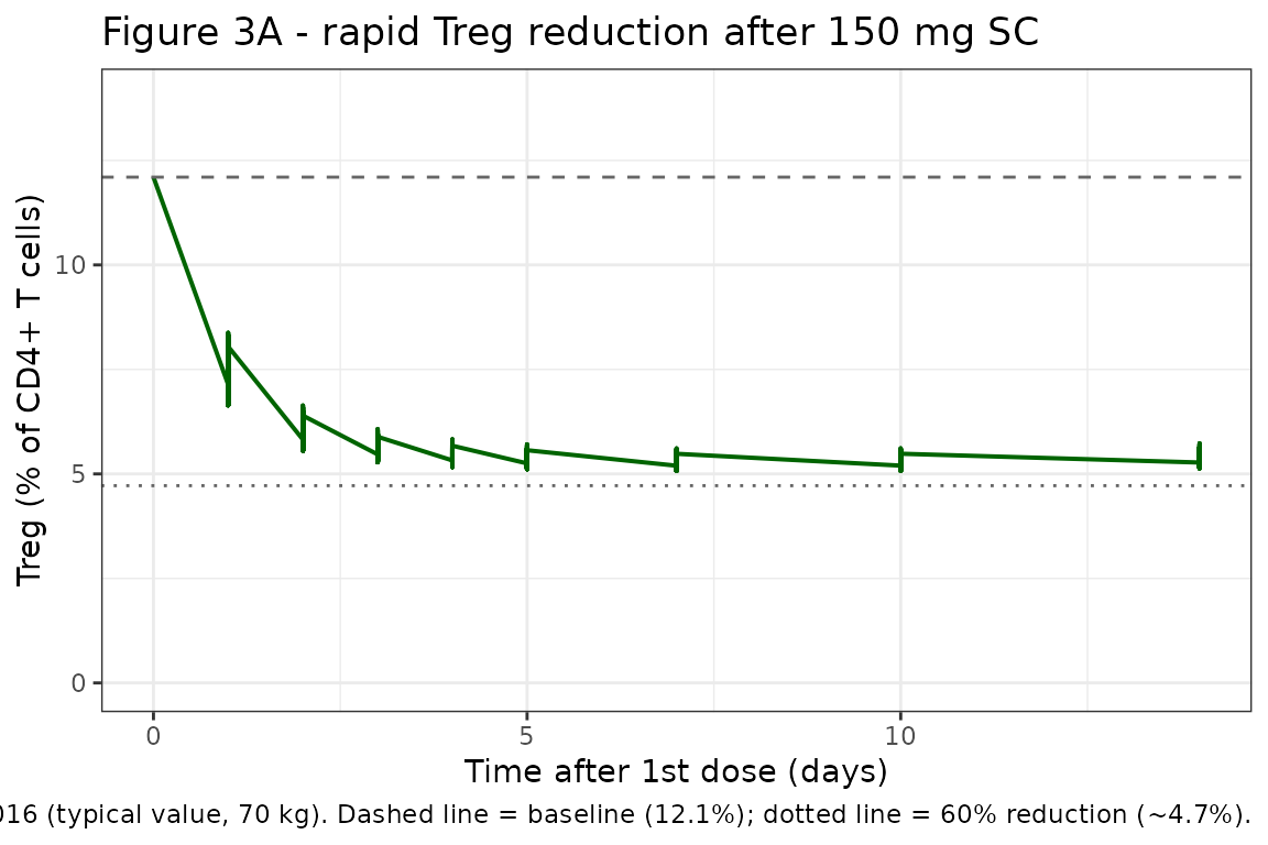

Figure 3B: Treg recovery after the last steady-state 150 mg SC dose

Diao 2016 Figure 3B shows return of Treg to baseline over ~20 weeks after the last steady-state 150 mg SC dose.

last_dose_t <- 140
fig3b <- sim_typ |>
  dplyr::filter(!is.na(treg), time >= last_dose_t) |>
  dplyr::distinct(id, time, .keep_all = TRUE) |>
  dplyr::mutate(weeks_after_last = (time - last_dose_t) / 7)

ggplot(fig3b, aes(weeks_after_last, treg)) +
  geom_line(color = "darkorange3", linewidth = 0.7) +
  geom_hline(yintercept = 12.1, linetype = "dashed", color = "grey40") +
  scale_y_continuous(limits = c(0, 14)) +
  labs(
    x = "Weeks after last dose",
    y = "Treg (% of CD4+ T cells)",
    title = "Figure 3B - Treg recovery after the last 150 mg SC dose",
    caption = "Replicates Figure 3B of Diao 2016. Dashed line = baseline (12.1%)."
  ) +
  theme_bw()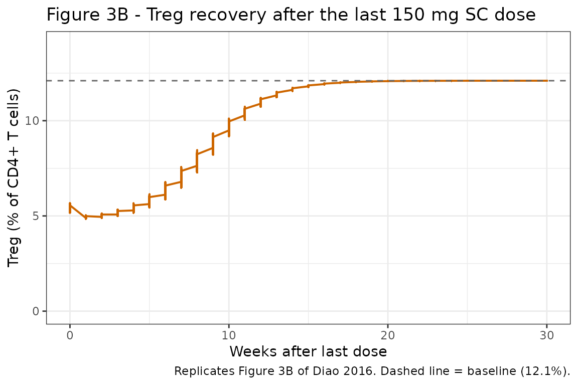

Stochastic VPC

vpc <- sim_pop |>
  dplyr::filter(!is.na(treg)) |>
  dplyr::distinct(id, time, .keep_all = TRUE) |>
  dplyr::group_by(time) |>
  dplyr::summarise(
    Q05 = quantile(treg, 0.05),
    Q50 = quantile(treg, 0.50),
    Q95 = quantile(treg, 0.95),
    .groups = "drop"
  )

ggplot(vpc, aes(time / 7, Q50)) +
  geom_ribbon(aes(ymin = Q05, ymax = Q95),
              fill = "darkgreen", alpha = 0.20) +
  geom_line(color = "darkgreen", linewidth = 0.7) +
  geom_hline(yintercept = 12.1, linetype = "dashed", color = "grey50") +
  labs(
    x = "Time (weeks)",
    y = "Treg (% of CD4+ T cells)",
    title = "Stochastic VPC: Treg by daclizumab HYP",
    caption = "5th-95th-percentile envelope across the virtual cohort."
  ) +
  theme_bw()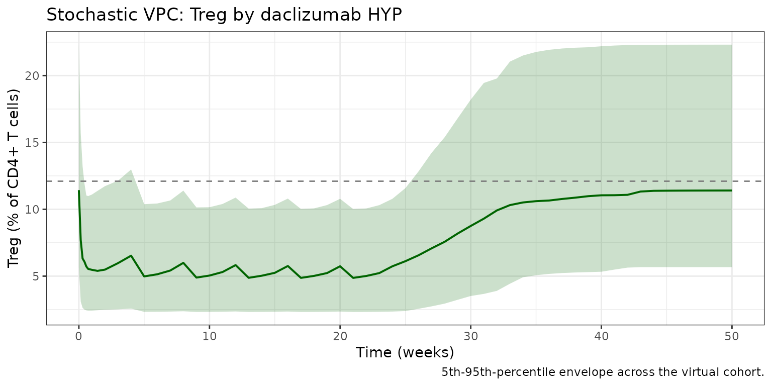

PKNCA validation (PK)

Treg percentage is not amenable to standard NCA. PKNCA is run on the inherited PK output to confirm steady-state (dose 5) Cmax / Cmin / AUC across one dosing interval.

sim_conc <- sim_pop |>
  dplyr::filter(!is.na(Cc), time >= 112, time <= 140) |>
  dplyr::distinct(id, time, .keep_all = TRUE) |>
  dplyr::mutate(time_in_interval = time - 112) |>
  dplyr::transmute(id = id, time = time_in_interval, Cc = Cc,
                   regimen = "150 mg SC Q4W")

dose_df <- events |>
  dplyr::filter(evid == 1, time == 112) |>
  dplyr::transmute(id = id, time = 0, amt = amt,
                   regimen = "150 mg SC Q4W")

conc_obj <- PKNCA::PKNCAconc(sim_conc, Cc ~ time | regimen + id)
dose_obj <- PKNCA::PKNCAdose(dose_df, amt ~ time | regimen + id)

intervals <- data.frame(
  start = 0, end = 28,
  cmax = TRUE, cmin = TRUE,
  tmax = TRUE, auclast = TRUE
)

nca <- PKNCA::pk.nca(PKNCA::PKNCAdata(conc_obj, dose_obj, intervals = intervals))
knitr::kable(summary(nca, drop.group = "id"),
             caption = "Steady-state (dose 5) NCA, 150 mg SC Q4W.")
#> Warning: The `drop.group` argument of `summary.PKNCAresults()` is deprecated as of PKNCA
#> 0.11.0.
#> ℹ Please use the `drop_group` argument instead.
#> This warning is displayed once per session.
#> Call `lifecycle::last_lifecycle_warnings()` to see where this warning was
#> generated.

Steady-state (dose 5) NCA, 150 mg SC Q4W.
start	end	regimen	N	auclast	cmax	cmin	tmax
0	28	150 mg SC Q4W	100	506 [28.2]	23.1 [27.9]	12.8 [32.9]	7.00 [7.00, 7.00]

Comparison against published behaviour

Diao 2016 reports two narrative checkpoints for the Treg reduction model:

typ <- sim_typ |>
  dplyr::filter(!is.na(treg)) |>
  dplyr::distinct(id, time, .keep_all = TRUE)

# Maximum reduction within first 14 days post first dose.
first_window <- typ |> dplyr::filter(time >= 0, time <= 14)
min_treg <- min(first_window$treg, na.rm = TRUE)
t_min   <- first_window$time[which.min(first_window$treg)]
max_red <- (12.1 - min_treg) / 12.1

# Time to return within 20% of baseline (10% absolute) after last dose.
after_last <- typ |> dplyr::filter(time >= 140)
recover_t_w <- (after_last$time[which(after_last$treg > 0.95 * 12.1)[1]] - 140) / 7

cmp <- tibble(
  metric    = c("Time to maximum reduction post 150 mg SC (days)",
                "Maximum fractional Treg reduction post 150 mg SC",
                "Time to >95% baseline recovery after last dose (weeks)"),
  published = c("~4 days", "~60%", "~20 weeks"),
  simulated = c(sprintf("%.1f", t_min),
                sprintf("%.1f%%", 100 * max_red),
                sprintf("%.1f", recover_t_w))
)
knitr::kable(cmp, caption = "Treg reduction / recovery checkpoints.")

Treg reduction / recovery checkpoints.
metric	published	simulated
Time to maximum reduction post 150 mg SC (days)	~4 days	7.0
Maximum fractional Treg reduction post 150 mg SC	~60%	58.1%
Time to >95% baseline recovery after last dose (weeks)	~20 weeks	14.0

Errata

Several non-substantive PDF text-extraction artifacts (operators rendered as /C0, etc.) appear in the trimmed source; they are not paper errata. Two model-relevant ambiguities are documented:

Hill coefficient point estimate without precision indicator. Diao 2016 Table 5 lists gamma = 2 for the Treg model with no standard error, no (FIXED) tag, and a bootstrap 95% CI of 1.39 to 2.91. The bootstrap CI is wide enough to encompass gamma = 1 (a hyperbolic Emax), but the Table 5 row format (no SE column populated alongside the value) is consistent with the value being treated as a fixed structural parameter during fitting. The library encodes treggamma <- fixed(2) to match.
Residual additive error units. Diao 2016 Table 5 reports “Residual error (additive): 0.416” with no explicit unit string. The Treg measurement scale is “% of CD4+ T cells” (per Table 5 baseline row), so the additive residual error is interpreted here as 0.416 percentage points; the proportional component (50.1%) is taken as a CV on the same scale (tregpropSd <- 0.501).

Assumptions and deviations

PK backbone is Othman 2014, not the in-paper PK summary. Same as the companion CD25 and CD56 bright vignettes: Diao 2016 fixed PK to a published RRMS PopPK model (CL = 0.212 L/day at 68 kg, allometric exponents 0.87 / 1.12, F = 0.88, t1/2,abs ~ 5 days, Tlag = 1.61 h) whereas the packaged PD model uses Othman 2014 healthy-volunteer PK (CL = 0.24 L/day at 70 kg, exponents 0.54 / 0.64, F = 0.84, ka = 0.216 /day, Tlag = 2 h). The IC50 of 3.97 mg/L is comparable to the typical clinical Cc range, so simulated Treg curves are sensitive to the PK assumption. Users who need exact reproduction of Diao 2016 Figure 3 numerical values can override the inherited PK ini() entries.
No PD covariates. Diao 2016 does not report covariate effects on the Treg PD parameters; only the inherited PK covariates (WT, DOSE_50MG) are present.
Hill coefficient treated as structurally fixed. See Errata.
Virtual-cohort weight distribution. Body weight is sampled from N(71, 14) kg truncated to 45-120 kg.