Torasemide in dogs (Pelligand 2020)
Source:vignettes/articles/Pelligand_2020_torasemide_dog.Rmd
Pelligand_2020_torasemide_dog.RmdModel and source
- Citation: Pelligand L, Guillot E, Geneteau A, Guyonnet J, Magnier R, Elliott J, Peyrou M, Jacobs M. Population Pharmacokinetics and Pharmacodynamics Modeling of Torasemide and Furosemide After Oral Repeated Administration in Healthy Dogs. Front Vet Sci. 2020;7:151. doi:10.3389/fvets.2020.00151.
- Description: Preclinical (beagle dog). Population PK/PD model for oral torasemide in healthy male Beagle dogs: two-compartment PK with first-order absorption (F fixed at 0.98) and a urinary-excretion arm carrying 61% of total clearance. The daily amount of torasemide excreted in urine drives (i) daily diuresis through a direct power model on top of a baseline urine output and (ii) natriuresis through an indirect-response model whose zero-order input is stimulated by a sigmoid Emax function; a threshold-activated reversible ‘diuretic resistance’ state reduces that Emax (Pelligand 2020)
- Article (open access): https://doi.org/10.3389/fvets.2020.00151
The model links oral torasemide pharmacokinetics in healthy Beagle
dogs to two pharmacodynamic endpoints through the amount of torasemide
excreted in urine (Aurine, in ug), which the authors found
to be a better driver than the plasma concentration because torasemide
acts from the luminal side of the loop of Henle:
-
Diuresis (daily urine volume, mL/day) – direct
power model,
urine_vol = Baseline + slope * Aurine^alpha(Equation 1). -
Natriuresis (daily urinary sodium, mEq/day) –
indirect-response model whose zero-order input
kforNais stimulated by a sigmoid Emax function ofAurine(Equations 2-6). A reversible “diuretic resistance” staternabuilds up at a zero-order rate whenever the fractional stimulation exceeds an estimated threshold, and scales the Emax down asEmax * (1 - rna)(Equations 7-8).
The furosemide arms of the study were not modelled.
Population
Two placebo-controlled crossover studies in healthy male Beagle dogs were pooled (Table 1 and Supplementary Table S1): study 1 (5 dogs, 9.3-11.6 kg, 1-2.1 years; once-daily oral torasemide 0.1, 0.2, 0.4 and 0.8 mg/kg for 14 days) and study 2 (12 dogs, 9.9-11.2 kg, 15-19 months; torasemide 0.1, 0.2, 0.3 and 0.4 mg/kg once daily on Day 1 and again on Days 5-14, plus four furosemide arms). Doses were given as tablets about 30 minutes after food. The 0.8 mg/kg period was excluded from the PK/PD analysis because renal tubular changes were seen at that dose in a safety study. For the PD analysis urine volumes, urinary sodium and urinary torasemide were summed over 24-h collection periods.
The same information is available programmatically via
readModelDb("Pelligand_2020_torasemide_dog")()$population.
Source trace
| Equation / parameter | Value | Source location |
|---|---|---|
lfdepot (F) |
0.98, fixed | Table 2; Methods ‘Pharmacokinetic Modeling’ |
lka |
1.66 1/h | Table 2 |
lcl |
0.077 L/h | Table 2 |
lfe (Fu) |
0.611 | Table 2 |
lvc |
0.145 L | Table 2 |
lq |
0.262 L/h | Table 2 |
lvp |
0.935 L | Table 2 |
lurprod (Baseline) |
221 mL/day | Table 3 |
lslope |
10^-4.11 mL/ug^alpha | Table 3; Methods ‘PK/PD modeling of diuresis’ |
lalpha |
2.05 | Table 3 |
lkin (kforNa) |
3.67 mEq/h^2 | Table 4 |
lkout (kabsNa) |
4.99 1/h | Table 4 |
lemax |
4.67 | Table 4 |
lec50 |
1080 ug | Table 4 |
lhill |
2.57 | Table 4 |
lkres_on |
0.0811 1/h | Table 4 |
lkres_off |
0.0894 1/h | Table 4 |
lres_thres |
0.0547 | Table 4; Results ‘PK/PD Modeling of Torasemide-Induced Natriuresis’ |
IIV (etalka, etalcl,
etalfe) |
126.1%, 64.3%, 8.6% CV | Table 2 |
IIV (etalurprod, etalslope,
etalalpha) |
13.4%, 45.8%, 3.9% CV | Table 3 |
IIV (etalkin, etalemax) |
19.4%, 62.4% CV | Table 4 |
propSd (plasma) |
18.4% | Table 2 |
propSd_Aurine, addSd_Aurine
|
22.5%, 3.68 ug | Table 2 |
propSd_urine_vol |
43.2% | Table 3 |
propSd_qna |
30.5% | Table 4 |
Two-compartment PK with urinary arm fe * CL
|
– | Figure 1; Results ‘Pharmacokinetic Model’ |
urine_vol = Baseline + slope * Aurine^alpha |
– | Equation 1 |
d/dt(qna) = ena |
– | Equation 2 |
ena(0) = kforNa / kabsNa |
– | Equation 4 |
ena_tora sigmoid Emax on Aurine
|
– | Equation 5 |
d/dt(ena) = kforNa * (1 + ena_tora) - kabsNa * ena |
– | Equation 6 |
d/dt(rna) = kResON - kResOFF * rna, kResON = 0 below
threshold |
– | Equation 7 and text |
Emax_apparent = Emax * (1 - rna) |
– | Equation 8 |
IIV variances were converted from the published CV% with
omega^2 = log(1 + CV^2), the inverse of the conversion the
Methods print.
Virtual cohort and simulation
The simulation follows the study 2 design: torasemide 0.1, 0.2, 0.3
or 0.4 mg/kg once daily on Day 1 (t = 0 h) and Days 5-14 (t = 96-312 h),
100 dogs per arm, body weight drawn uniformly over the study 2 range
(9.9-11.2 kg). Body weight is not a model covariate; it only converts
the mg/kg dose to the absolute mg dose the model expects. The urinary
compartments urine and qna are reset to zero
at the end of every 24-h collection with an evid = 5
replacement record placed a numerical epsilon after the boundary, so the
end-of-collection observation at exactly 24, 48, … h reads the full
daily amount before the reset.
mod <- readModelDb("Pelligand_2020_torasemide_dog")
doses_mgkg <- c(0.1, 0.2, 0.3, 0.4)
dose_times <- c(0, seq(96, 312, by = 24)) # Day 1 and Days 5-14
day_ends <- 24 * (1:17)
pk_grid <- c(0, 0.25, 0.5, 0.75, 1, 1.5, 2, 4, 6, 8, 12)
pk_times <- c(pk_grid, 24, 312 + c(pk_grid, 24, 36, 48, 60, 72, 96))
obs_times <- sort(unique(c(pk_times, day_ends)))

make_arm <- function(n, dose_mgkg, wt, id_offset) {
  ids <- id_offset + seq_len(n)
  dose <- data.frame(
    id = rep(ids, each = length(dose_times)),
    time = rep(dose_times, n),
    amt = rep(dose_mgkg * wt, each = length(dose_times)),
    evid = 1L, cmt = "depot", dvid = NA_integer_
  )
  reset <- expand.grid(time = day_ends + 1e-6, cmt = c("urine", "qna"), id = ids,
                       stringsAsFactors = FALSE)
  reset$amt <- 0
  reset$evid <- 5L
  reset$dvid <- NA_integer_
  obs <- expand.grid(time = obs_times, id = ids)
  obs$amt <- NA_real_
  obs$evid <- 0L
  obs$cmt <- "central"
  obs$dvid <- 1L
  out <- dplyr::bind_rows(dose, reset, obs)
  out$dose_mgkg <- dose_mgkg
  dplyr::arrange(out, id, time)
}

set.seed(20200428)
n_per_arm <- 100
arms <- lapply(seq_along(doses_mgkg), function(k) {
  wt <- stats::runif(n_per_arm, 9.9, 11.2)
  make_arm(n_per_arm, doses_mgkg[k], wt, id_offset = (k - 1) * n_per_arm)
})
# method = "dop853": with a 126% CV on ka and a threshold switch in the
# resistance equation, the default liblsoda (and lsoda) fail to solve roughly a
# third of the simulated dogs; the explicit Runge-Kutta solver solves them all.
sim <- dplyr::bind_rows(lapply(seq_along(arms), function(k) {
  rxode2::rxSetSeed(100 + k)
  s <- rxode2::rxSolve(mod, arms[[k]], returnType = "data.frame",
                       keep = "dose_mgkg", maxsteps = 100000L, method = "dop853")
  s
}))
#> ℹ parameter labels from comments will be replaced by 'label()'
sim$treatment <- paste(sim$dose_mgkg, "mg/kg/day")
stopifnot(!anyNA(sim$Cc), !anyNA(sim$qna)) # every simulated dog solved

# Typical-value (no IIV, no residual error) solve for a 10.6 kg dog, the study 2
# mean body weight. omega = NA / sigma = NA gives the typical subject.
typ_events <- dplyr::bind_rows(lapply(seq_along(doses_mgkg), function(k) {
  make_arm(1, doses_mgkg[k], 10.6, id_offset = k - 1)
}))
typ <- rxode2::rxSolve(mod, typ_events, omega = NA, sigma = NA,
                       returnType = "data.frame", keep = "dose_mgkg",
                       method = "dop853")
typ$treatment <- paste(typ$dose_mgkg, "mg/kg/day")
daily_typ <- typ |>
  dplyr::filter(time %in% day_ends) |>
  dplyr::mutate(day = time / 24)
Replicate published figures
Plasma torasemide (Figure 3)
pk_plot <- sim |>
  dplyr::filter(time %in% pk_times) |>
  dplyr::group_by(treatment, time) |>
  dplyr::summarise(med = median(Cc), lo = quantile(Cc, 0.05), hi = quantile(Cc, 0.95),
                   .groups = "drop") |>
  dplyr::filter(med > 1)
ggplot(pk_plot, aes(time / 24, med, colour = treatment, fill = treatment)) +
  geom_ribbon(aes(ymin = lo, ymax = hi), alpha = 0.15, colour = NA) +
  geom_line() +
  scale_y_log10() +
  labs(x = "Time (day)", y = "Plasma torasemide (ug/L)", colour = NULL, fill = NULL) +
  theme_bw()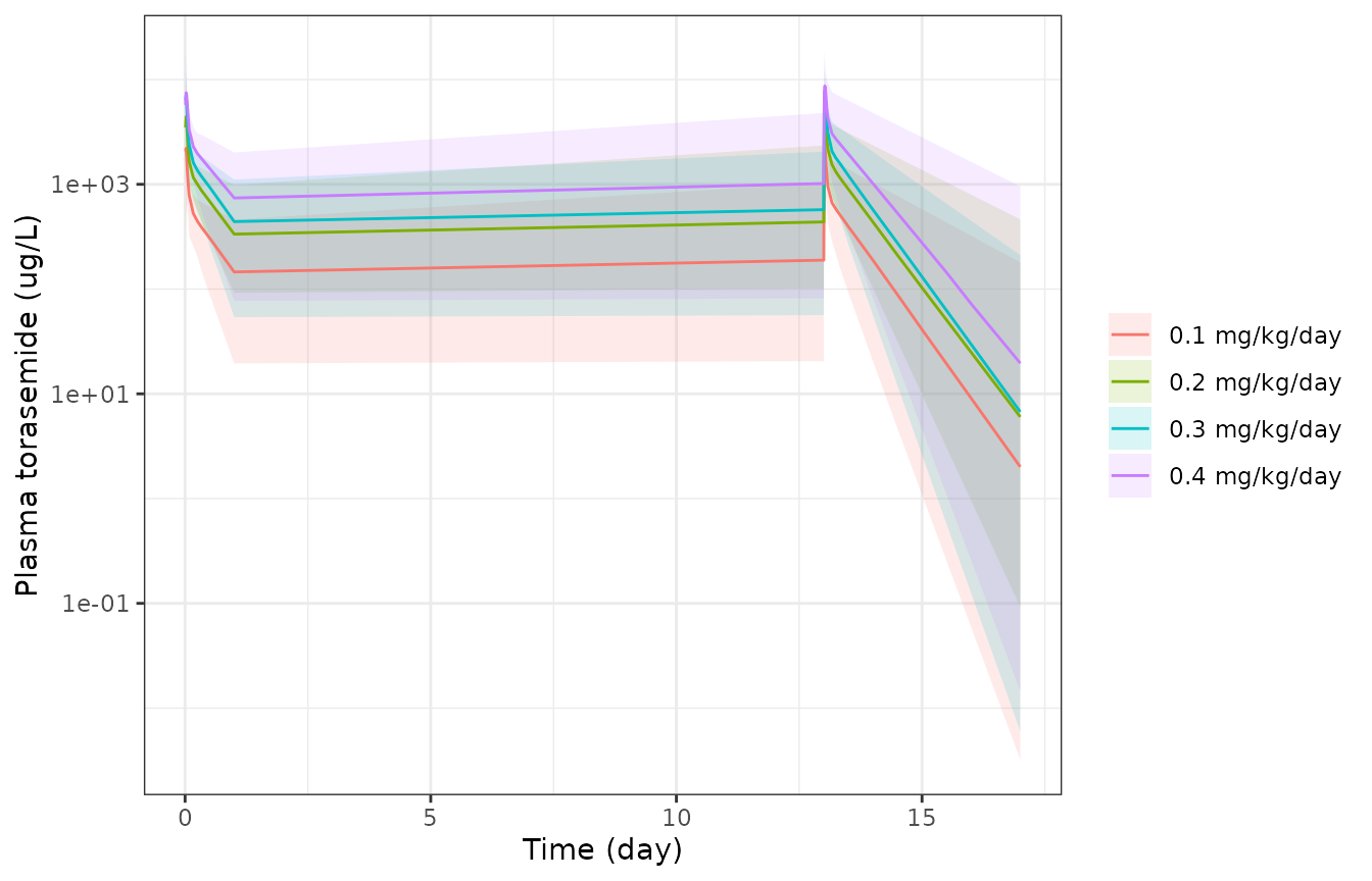
Replicates Figure 3 of Pelligand 2020: plasma torasemide after Day 1 and after the last (Day 14) dose, study 2. Lines are simulated medians; ribbons the 5th-95th percentiles.
The simulated concentrations sit above the mean observed profiles of Figures 2 and 3 and decline more slowly: at 0.4 mg/kg/day the figures show mean peaks of roughly 3000-4000 ug/L and a 24-h value of roughly 250-400 ug/L, while the typical dog of the published parameters peaks near 9000 ug/L and is still about 650 ug/L at 24 h. This is a property of the published model rather than of the implementation. Table 2 gives CL = 0.077 L/h and a central volume of only 0.145 L, so the typical AUC over a dosing interval is dose x F / CL (about 53 mg.h/L at 0.4 mg/kg in a 10.6 kg dog), and the paper’s own diagnostic plot of conditional weighted residuals against population predictions (Supplementary Figure S2) spans population predictions up to about 9500 ug/L, the value the typical dog reaches here after the last 0.4 mg/kg dose. The large absorption variability (126% CV on ka) also flattens the mean of the observed profiles relative to the typical curve.
Daily urinary torasemide (Figure 4)
daily_sim <- sim |>
  dplyr::filter(time %in% day_ends) |>
  dplyr::mutate(day = time / 24)
daily_sim |>
  dplyr::group_by(treatment, day) |>
  dplyr::summarise(Aurine = median(Aurine), .groups = "drop") |>
  ggplot(aes(day, Aurine, colour = treatment)) +
  geom_line() + geom_point() +
  labs(x = "Day", y = "Urinary torasemide per 24 h (ug)", colour = NULL) +
  theme_bw()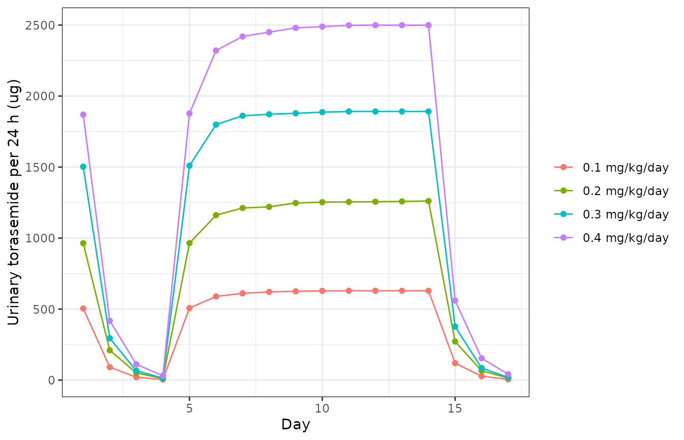
Replicates Figure 4 of Pelligand 2020: torasemide amount excreted in urine per 24-h collection, study 2 design. Simulated median per day.
Figure 4 of the paper shows mean daily urinary torasemide of roughly 520, 980, 1580 and 2170 ug on Day 1 and plateaus of roughly 590, 1180, 1850 and 2630 ug on Days 6-14 for 0.1-0.4 mg/kg/day (values read from the figure by the maintainers). The typical dog reproduces them:
fig4 <- tibble::tribble(
  ~dose_mgkg, ~day, ~published,
  0.1, 1, 520, 0.2, 1, 980, 0.3, 1, 1580, 0.4, 1, 2170,
  0.1, 10, 590, 0.2, 10, 1180, 0.3, 10, 1850, 0.4, 10, 2630
)
urine_cmp <- fig4 |>
  dplyr::left_join(daily_typ |> dplyr::select(dose_mgkg, day, Aurine),
                   by = c("dose_mgkg", "day")) |>
  dplyr::mutate(pct_diff = 100 * (Aurine - published) / published)
urine_cmp |>
  dplyr::mutate(Aurine = round(Aurine), pct_diff = round(pct_diff, 1)) |>
  dplyr::rename("Dose (mg/kg/day)" = dose_mgkg, "Day" = day,
                "Figure 4 (ug)" = published, "Typical simulated (ug)" = Aurine,
                "Difference (%)" = pct_diff) |>
knitr::kable()| Dose (mg/kg/day) | Day | Figure 4 (ug) | Typical simulated (ug) | Difference (%) |
|---|---|---|---|---|
| 0.1 | 1 | 520 | 503 | -3.4 |
| 0.2 | 1 | 980 | 1005 | 2.6 |
| 0.3 | 1 | 1580 | 1508 | -4.6 |
| 0.4 | 1 | 2170 | 2010 | -7.4 |
| 0.1 | 10 | 590 | 635 | 7.6 |
| 0.2 | 10 | 1180 | 1269 | 7.6 |
| 0.3 | 10 | 1850 | 1904 | 2.9 |
| 0.4 | 10 | 2630 | 2538 | -3.5 |
Diuresis (Figure 5 and Table 5)
diur_pub <- tibble::tribble(
  ~dose_mgkg, ~day, ~published, ~source,
  0.3, 1, 512, "Results text (first administration)",
  0.4, 1, 638, "Results text (first administration)",
  0.1, 9, 220, "Table 5 (Day 9)",
  0.2, 9, 403, "Table 5 (Day 9)",
  0.3, 9, 773, "Table 5 (Day 9)",
  0.4, 9, 1150, "Table 5 (Day 9)"
)
diur_cmp <- diur_pub |>
  # Table 5 'D9' is the late repeated-dose steady state (the Results give the
  # same 773 / 1150 mL as 'after the 10th dose'); study day 13 is used.
  dplyr::mutate(day_sim = ifelse(day == 1, 1, 13)) |>
  dplyr::left_join(daily_typ |> dplyr::select(dose_mgkg, day, urine_vol),
                   by = c("dose_mgkg", day_sim = "day")) |>
  dplyr::mutate(pct_diff = 100 * (urine_vol - published) / published)
diur_cmp |>
  dplyr::transmute(dose_mgkg, source, published, urine_vol = round(urine_vol),
                   pct_diff = round(pct_diff, 1)) |>
  dplyr::rename("Dose (mg/kg/day)" = dose_mgkg, "Source" = source,
                "Published (mL/day)" = published,
                "Typical simulated (mL/day)" = urine_vol,
                "Difference (%)" = pct_diff) |>
knitr::kable()| Dose (mg/kg/day) | Source | Published (mL/day) | Typical simulated (mL/day) | Difference (%) |
|---|---|---|---|---|
| 0.3 | Results text (first administration) | 512 | 475 | -7.2 |
| 0.4 | Results text (first administration) | 638 | 680 | 6.5 |
| 0.1 | Table 5 (Day 9) | 220 | 264 | 20.1 |
| 0.2 | Table 5 (Day 9) | 403 | 400 | -0.8 |
| 0.3 | Table 5 (Day 9) | 773 | 632 | -18.3 |
| 0.4 | Table 5 (Day 9) | 1150 | 961 | -16.4 |
# First-administration diuresis at the two highest doses is the cleanest
# structural check (no time-dependent drift, see below).
stopifnot(abs(diur_cmp$pct_diff[diur_cmp$day == 1]) < 15)
# Baseline urine output (Table 3: 221 mL/day; Results: 220 mL/day).
stopifnot(abs(exp(rxode2::rxode(mod)$theta[["lurprod"]]) - 220) / 220 < 0.05)
#> ℹ parameter labels from comments will be replaced by 'label()'
The first-administration diuresis at 0.3 and 0.4 mg/kg/day is reproduced within a few percent. The Day 9 values at 0.3 and 0.4 mg/kg/day are under-predicted by 16-18%: the paper reports that at doses of 0.3 mg/kg/day and above the daily urine volume kept increasing over the 10 treatment days although the urinary torasemide amount stayed constant, a time-dependent increase the direct power model cannot express (it predicts the same volume for the same daily urinary amount). The 0.1 mg/kg/day Day 9 value is over-predicted by about 20% in absolute terms of ~40 mL/day.
daily_sim |>
  dplyr::group_by(treatment, day) |>
  dplyr::summarise(med = median(urine_vol), lo = quantile(urine_vol, 0.05),
                   hi = quantile(urine_vol, 0.95), .groups = "drop") |>
  ggplot(aes(day, med, colour = treatment, fill = treatment)) +
  geom_ribbon(aes(ymin = lo, ymax = hi), alpha = 0.1, colour = NA) +
  geom_line() + geom_point() +
  labs(x = "Day", y = "Urine volume per 24 h (mL)", colour = NULL, fill = NULL) +
  theme_bw()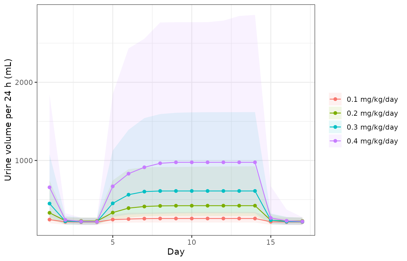
Replicates Figure 6 of Pelligand 2020 (torasemide arms): daily urine volume, study 2 design. Lines are simulated medians.
Dose-response for diuresis (Figure 10)
The paper selected 0.26 mg/kg/day as the dose giving a target daily diuresis of 460 mL and 0.13 mg/kg/day as the dose giving 284 mL/day (Discussion), both read from the typical-parameter dose-response of Figure 10. The typical steady-state daily diuresis for a 10.5 kg dog (the weight the Discussion uses) is:
dr_doses <- seq(0.05, 0.45, by = 0.01)
dr_events <- dplyr::bind_rows(lapply(seq_along(dr_doses), function(k) {
  make_arm(1, dr_doses[k], 10.5, id_offset = k - 1)
}))
dr <- rxode2::rxSolve(mod, dr_events, omega = NA, sigma = NA,
                      returnType = "data.frame", keep = "dose_mgkg",
                      method = "dop853") |>
  dplyr::filter(time == 13 * 24) # Day 9 of repeated dosing (steady state)
ggplot(dr, aes(dose_mgkg, urine_vol)) +
  geom_line() +
  geom_hline(yintercept = c(284, 460), linetype = 2) +
  geom_vline(xintercept = c(0.13, 0.26), linetype = 3) +
  labs(x = "Torasemide dose (mg/kg/day)", y = "Daily diuresis (mL/day)") +
  theme_bw()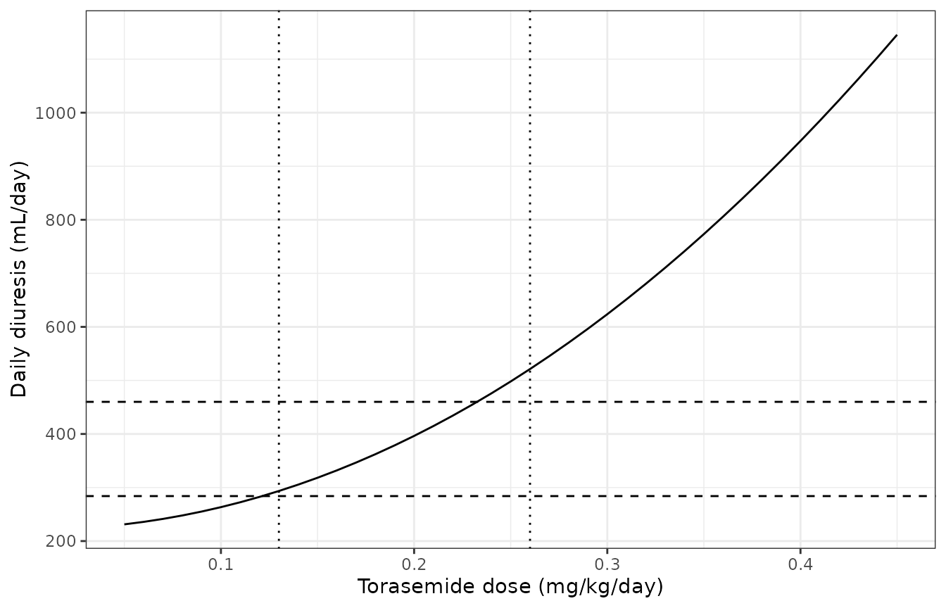
dr_cmp <- tibble::tibble(dose_mgkg = c(0.13, 0.26), published = c(284, 460)) |>
  dplyr::left_join(dr |> dplyr::mutate(dose_mgkg = round(dose_mgkg, 2)) |>
                     dplyr::select(dose_mgkg, urine_vol), by = "dose_mgkg") |>
  dplyr::mutate(pct_diff = 100 * (urine_vol - published) / published)
dr_cmp |>
  dplyr::mutate(urine_vol = round(urine_vol), pct_diff = round(pct_diff, 1)) |>
  dplyr::rename("Dose (mg/kg/day)" = dose_mgkg, "Discussion (mL/day)" = published,
                "Typical simulated (mL/day)" = urine_vol,
                "Difference (%)" = pct_diff) |>
knitr::kable()| Dose (mg/kg/day) | Discussion (mL/day) | Typical simulated (mL/day) | Difference (%) |
|---|---|---|---|
| 0.13 | 284 | 294 | 3.3 |
| 0.26 | 460 | 521 | 13.3 |
The low dose is reproduced within a few percent; at 0.26 mg/kg/day the typical steady-state diuresis is about 13% above the published 460 mL/day. The paper does not state the body weight, treatment day or dose grid used in its Berkeley Madonna simulation, and the two published doses were read off a curve, so a residual difference of this size is expected.
Natriuresis (Figures 7, 8 and S12)
daily_sim |>
  dplyr::group_by(treatment, day) |>
  dplyr::summarise(med = median(qna), lo = quantile(qna, 0.05),
                   hi = quantile(qna, 0.95), .groups = "drop") |>
  ggplot(aes(day, med, colour = treatment, fill = treatment)) +
  geom_ribbon(aes(ymin = lo, ymax = hi), alpha = 0.1, colour = NA) +
  geom_line() + geom_point() +
  labs(x = "Day", y = "Sodium excreted per 24 h (mEq)", colour = NULL, fill = NULL) +
  theme_bw()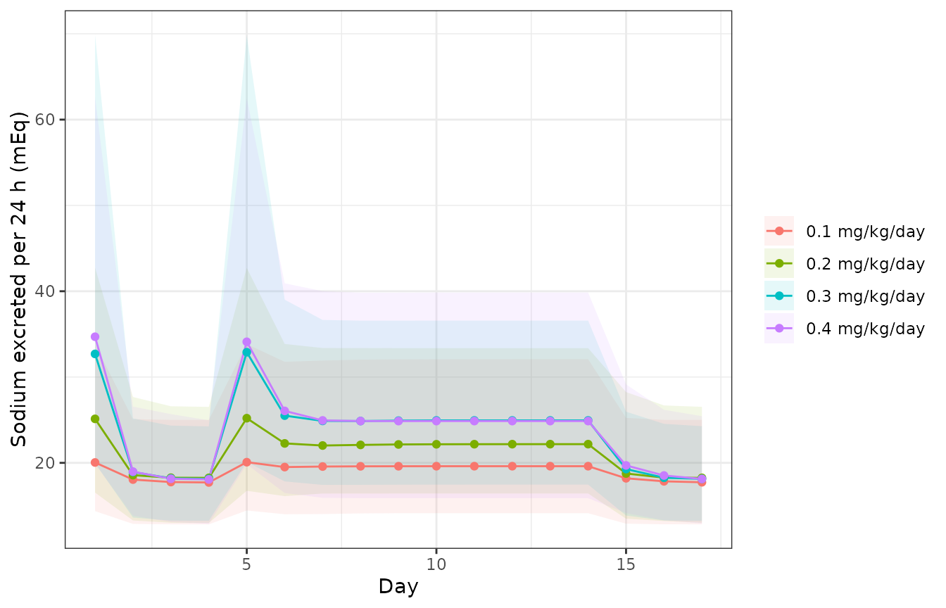
Replicates Figure 8 of Pelligand 2020 (torasemide arms): daily urinary sodium, study 2 design. Lines are simulated medians; ribbons the 5th-95th percentiles.
na_pub <- tibble::tribble(
  ~dose_mgkg, ~published_d1, ~published_rep,
  0.1, 23.5, 15.0,
  0.2, 30.7, 19.7,
  0.3, 42.2, 24.7,
  0.4, 56.6, 31.7
)
na_cmp <- na_pub |>
  dplyr::left_join(daily_typ |> dplyr::filter(day == 1) |>
                     dplyr::select(dose_mgkg, sim_d1 = qna), by = "dose_mgkg") |>
  dplyr::left_join(daily_typ |> dplyr::filter(day == 13) |>
                     dplyr::select(dose_mgkg, sim_rep = qna), by = "dose_mgkg")
na_cmp |>
  dplyr::mutate(dplyr::across(c(sim_d1, sim_rep), ~ round(.x, 1))) |>
  dplyr::rename("Dose (mg/kg/day)" = dose_mgkg,
                "First dose, Figure 7" = published_d1,
                "First dose, typical simulated" = sim_d1,
                "Repeated dose, Figure 7" = published_rep,
                "Repeated dose, typical simulated" = sim_rep) |>
knitr::kable(caption = "Daily urinary sodium (mEq/day). Published values read from Figure 7 by the maintainers; 0.4 mg/kg first dose = 56.6 mEq/day in the Results text.")| Dose (mg/kg/day) | First dose, Figure 7 | Repeated dose, Figure 7 | First dose, typical simulated | Repeated dose, typical simulated |
|---|---|---|---|---|
| 0.1 | 23.5 | 15.0 | 19.6 | 19.5 |
| 0.2 | 30.7 | 19.7 | 25.3 | 22.0 |
| 0.3 | 42.2 | 24.7 | 31.9 | 23.7 |
| 0.4 | 56.6 | 31.7 | 37.2 | 24.7 |
# Baseline natriuresis kforNa / kabsNa x 24 h against the Results' 16 mEq/day.
na_base <- 24 * exp(rxode2::rxode(mod)$theta[["lkin"]] - rxode2::rxode(mod)$theta[["lkout"]])
#> ℹ parameter labels from comments will be replaced by 'label()'
#> ℹ parameter labels from comments will be replaced by 'label()'
na_base
#> [1] 17.6513
stopifnot(abs(na_base - 16) / 16 < 0.15)
# Resistance: the daily natriuresis falls from the first-dose peak to a lower
# repeated-dose plateau at every dose that activates it.
stopifnot(all(na_cmp$sim_rep < na_cmp$sim_d1))
The typical dog reproduces the baseline natriuresis (17.6 vs 16 mEq/day) and the collapse of natriuresis from the first-dose peak to a repeated-dose plateau. The first-dose values are under-predicted at every dose, by about 4-5 mEq/day at 0.1-0.2 mg/kg/day and increasingly at 0.3 and 0.4 mg/kg/day (about 32 and 37 mEq/day against 42 and 57). The repeated-dose plateau is flatter across doses than observed (about 20-25 mEq/day against 15-32). The paper’s own natriuresis VPC (Supplementary Figure S12, pooled over the four doses) shows the same first-day under-prediction: its predicted median rises only to about 22 mEq/day on the first day of repeated dosing while observations reach 70 mEq/day. The pooled simulated median below follows the shape of that VPC – a first-day peak, a plateau a few mEq/day above baseline, and a return towards baseline after the last dose – and sits 2-5 mEq/day above it, close to the offset of the baseline (17.6 mEq/day from Table 4 against the VPC’s ~16.5).
vpc <- daily_sim |>
  dplyr::filter(time >= 96) |>
  dplyr::mutate(sim_obs = qna * (1 + stats::rnorm(dplyr::n(), 0, 0.305))) |>
  dplyr::group_by(time) |>
  dplyr::summarise(med = median(qna), lo = quantile(sim_obs, 0.05),
                   hi = quantile(sim_obs, 0.95), .groups = "drop")
ggplot(vpc, aes(time, med)) +
  geom_ribbon(aes(ymin = lo, ymax = hi), fill = "grey80") +
  geom_line(linewidth = 1) +
  labs(x = "Time (h)", y = "Sodium excreted over 24 h (mEq)") +
  theme_bw()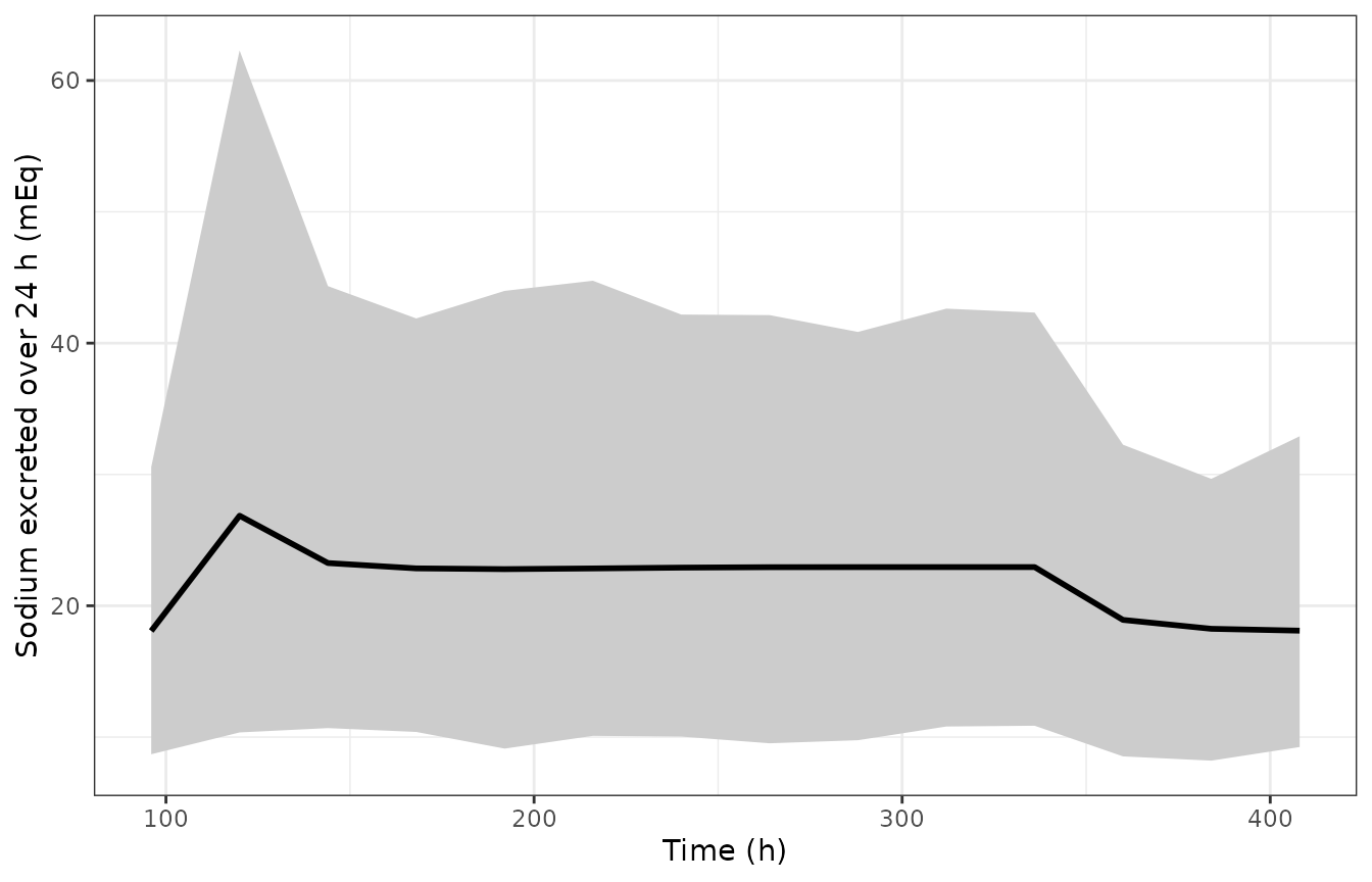
Replicates Supplementary Figure S12 of Pelligand 2020: VPC of daily urinary sodium pooled over 0.1-0.4 mg/kg/day, Days 4-17 (x = end of each 24-h collection).
vpc_med <- setNames(vpc$med, vpc$time)
round(vpc_med[c("120", "144", "240", "336", "360", "384")], 1)
#>  120  144  240  336  360  384
#> 26.9 23.3 22.9 22.9 18.9 18.2
# Figure S12 predicted median: ~22 mEq at 120 h, ~20 on the plateau, back to
# ~16.5-17.5 after the last dose. Robust envelope, not the extreme.
stopifnot(
  vpc_med[["120"]] > 18, vpc_med[["120"]] < 32,
  vpc_med[["240"]] > 17, vpc_med[["240"]] < 26,
  vpc_med[["384"]] < vpc_med[["240"]]
)
PKNCA validation
The paper reports no NCA table. Its text gives a Tmax of 0.5-1 h after oral dosing (Abstract), an absorption half-life of 25 min (Discussion; ln 2 / 1.66 = 0.42 h) and an elimination half-life of “around 6 h” measured with results not shown (Discussion). NCA of the simulated Day 1 (0-24 h) and last-dose (Day 14, 312-408 h) profiles:
sim_nca <- sim |>
  dplyr::filter(!is.na(Cc), time %in% pk_times) |>
  dplyr::select(id, time, Cc, treatment)
sim_nca <- dplyr::bind_rows(
  sim_nca,
  sim_nca |> dplyr::distinct(id, treatment) |> dplyr::mutate(time = 0, Cc = 0)
) |>
  dplyr::distinct(id, treatment, time, .keep_all = TRUE) |>
  dplyr::arrange(id, treatment, time)

dose_df <- dplyr::bind_rows(arms) |>
  dplyr::filter(evid == 1) |>
  dplyr::mutate(treatment = paste(dose_mgkg, "mg/kg/day")) |>
  dplyr::select(id, time, amt, treatment)

conc_obj <- PKNCA::PKNCAconc(sim_nca, Cc ~ time | treatment + id)
dose_obj <- PKNCA::PKNCAdose(dose_df, amt ~ time | treatment + id)
intervals <- data.frame(
  start = c(0, 312), end = c(24, 408),
  cmax = TRUE, tmax = TRUE, auclast = c(TRUE, FALSE), half.life = c(FALSE, TRUE)
)
nca_res <- PKNCA::pk.nca(PKNCA::PKNCAdata(conc_obj, dose_obj, intervals = intervals))

nca_tbl <- as.data.frame(nca_res) |>
  dplyr::filter(PPTESTCD %in% c("cmax", "tmax", "auclast", "half.life")) |>
  dplyr::group_by(treatment, start, PPTESTCD) |>
  dplyr::summarise(median = signif(median(PPORRES, na.rm = TRUE), 3), .groups = "drop") |>
  tidyr::pivot_wider(names_from = PPTESTCD, values_from = median)
nca_tbl |>
  dplyr::rename("Treatment" = treatment, "Interval start (h)" = start,
                "Cmax (ug/L)" = cmax, "Tmax (h)" = tmax,
                "AUC0-24 (h*ug/L)" = auclast, "Half-life (h)" = half.life) |>
knitr::kable(caption = "Median simulated NCA parameters (Day 1: 0-24 h; last dose: 312-408 h).")| Treatment | Interval start (h) | AUC0-24 (h*ug/L) | Cmax (ug/L) | Tmax (h) | Half-life (h) |
|---|---|---|---|---|---|
| 0.1 mg/kg/day | 0 | 9760 | 2370 | 0.5 | NA |
| 0.1 mg/kg/day | 312 | NA | 2630 | 0.5 | 11.1 |
| 0.2 mg/kg/day | 0 | 21000 | 4420 | 0.5 | NA |
| 0.2 mg/kg/day | 312 | NA | 4990 | 0.5 | 11.8 |
| 0.3 mg/kg/day | 0 | 30500 | 7370 | 0.5 | NA |
| 0.3 mg/kg/day | 312 | NA | 7780 | 0.5 | 11.1 |
| 0.4 mg/kg/day | 0 | 43200 | 7590 | 0.5 | NA |
| 0.4 mg/kg/day | 312 | NA | 9240 | 0.5 | 12.7 |
published <- tibble::tibble(
  treatment = paste(doses_mgkg, "mg/kg/day"),
  tmax = 0.75 # Abstract: Tmax 0.5-1 h (midpoint)
)
cmp <- nlmixr2lib::ncaComparisonTable(
  simulated = nca_res,
  reference = published,
  by = "treatment",
  units = c(tmax = "h"),
  tolerance_pct = 50
)
knitr::kable(cmp, caption = "Simulated vs. published Tmax (published: 0.5-1 h, compared at its 0.75 h midpoint). * differs by >50%.")| NCA parameter | treatment | Reference | Simulated | % diff |
|---|---|---|---|---|
| Tmax (h) | 0.1 mg/kg/day | 0.75 | 0.5 | -33.3% |
| Tmax (h) | 0.2 mg/kg/day | 0.75 | 0.5 | -33.3% |
| Tmax (h) | 0.3 mg/kg/day | 0.75 | 0.5 | -33.3% |
| Tmax (h) | 0.4 mg/kg/day | 0.75 | 0.5 | -33.3% |
tmax_d1 <- as.data.frame(nca_res) |>
  dplyr::filter(PPTESTCD == "tmax", start == 0)
stopifnot(dplyr::between(median(tmax_d1$PPORRES), 0.5, 1))
The simulated median Tmax falls inside the published 0.5-1 h range. The simulated terminal half-life over 312-408 h is longer than the “around 6 h” quoted in the Discussion: the published two-compartment disposition (Table 2) has a slow terminal phase (terminal rate constant 0.058 1/h, half-life about 12 h) that carries a small fraction of the AUC, and the Discussion’s figure was derived by a method the paper does not show. Plasma torasemide AUC in the paper was also less than dose-proportional-linear (power-model exponent 1.26-1.59), which the linear population model does not reproduce by construction.
Assumptions and deviations
-
Driver of the PD sub-models. The paper defines
Qurineas “the quantity of torasemide excreted in urine in ug per day” without saying whether, inside the natriuresis differential equation, it is the amount accumulated since the start of the current 24-h collection or the instantaneous urinary excretion rate scaled to a day. The maintainers implemented the accumulated amount (theurinecompartment reset at each 24-h boundary; Results: “The bladder was considered empty after each urination”), because (i) the diuresis equation uses the daily excreted amount directly, (ii) that reading reproduces the paper’s natriuresis VPC (Supplementary Figure S12) while the rate reading predicts a first-day median near 35 mEq/day, well above the VPC’s ~22, and- Table 4 expresses EC50 as an amount (ug).
-
Resistance threshold. The threshold is applied to
the fractional stimulation computed with the resistance-reduced Emax
(Equation 8 feeds Equation 6 through a single
ENaTora). Applying it to the stimulation with the unreduced Emax changes the repeated-dose plateau by less than 1 mEq/day. - IIV on the diuresis slope. Table 3 reports the slope on the log10 scale (-4.11) with a 45.8% CV. Applying an exponential random effect to the log10 value itself would scale the drug effect up to ~100-fold at one SD, which is incompatible with the 38-45% between-dog CV of diuresis the paper observed at 0.3-0.4 mg/kg/day. The random effect is therefore applied multiplicatively to the linear-scale slope (log-normal slope with 45.8% CV).
- Body weight. The PK parameters are absolute (L, L/h) for dogs of about 10 kg and the model has no body-weight covariate. The vignette doses mg/kg x body weight, with weights drawn over the study 2 range (typical dog 10.6 kg; 10.5 kg for the dose-response, as in the Discussion).
- Dose rounding. Dogs received 2, 4 and 8 mg tablets; the exact mg doses are not tabulated, so nominal mg/kg x weight doses are simulated.
- Figure-read values. The Figure 4, Figure 7 and Supplementary Figure S12 comparison values were read from the published figures by the maintainers.
- Furosemide arms and aldosterone data were reported but not modelled by the authors and are not part of this model.
- No erratum or correction notice for this article was found (checked 2026-09-26).