Daridorexant (Krause 2023)
Source:vignettes/articles/Krause_2023_daridorexant.Rmd
Krause_2023_daridorexant.RmdModel and source
- Citation: Krause A, Lott D, Brussee JM, Muehlan C, Dingemanse J. (2023). Population pharmacokinetic modeling of daridorexant, a novel dual orexin receptor antagonist. CPT: Pharmacometrics & Systems Pharmacology 12(1):74-86. doi:10.1002/psp4.12877.
- Description: Two-compartment population PK model for oral daridorexant (a dual orexin receptor antagonist) in 1898 healthy subjects and patients with insomnia disorder pooled from 13 phase 1, two phase 2 and two phase 3 studies (Krause 2023). First-order absorption after a lag time; Michaelis-Menten elimination from the central compartment. Relative bioavailability decreases with dose (power, referenced to 50 mg). Food status (fasted or high-fat, high-calorie meal versus a light meal / uncontrolled food intake) acts on the lag time and ka, and morning versus bedtime dosing on ka. Lean body weight scales the central volume, fat mass the peripheral volume and the intercompartmental clearance, and age, alkaline phosphatase and lean body weight scale Km. Log-normal IIV on all eight structural parameters, inter-occasion variability on F, the lag time and ka, and a combined additive + proportional residual error.
- Article (open access): https://doi.org/10.1002/psp4.12877
Daridorexant is a dual orexin receptor antagonist for insomnia, dosed at bedtime. Krause 2023 pooled 13 phase 1, two phase 2 and two phase 3 studies into one Monolix (SAEM) population PK model: two compartments, first-order absorption after a lag time, Michaelis-Menten elimination and a relative bioavailability that falls with dose. The paper reports one final model, so the package carries one model file.
Population
The phase 1 studies contributed 9420 concentrations from 412 subjects with dense sampling (healthy subjects and subjects with hepatic or renal impairment); the two phase 2 and two phase 3 studies contributed 3207 next-morning concentrations from 1486 patients with insomnia disorder, 12 627 concentrations from 1898 subjects in total (Results, Data characteristics). Subjects were 18-88 years old (median 54), weighed 42-119.5 kg (median 73.6), had a lean body weight of 29.1-83.9 kg (median 47.2) and a fat mass of 7.0-58.6 kg (median 23.4); 1155 were female and 1646 White (Table 1). Oral doses ranged from 5 to 200 mg. Phase 1 subjects were mostly dosed in the morning, phase 2 and 3 patients at bedtime.
str(rxode2::rxode(readModelDb("Krause_2023_daridorexant"))$population)
#> ℹ parameter labels from comments will be replaced by 'label()'
#> Warning: some etas defaulted to non-mu referenced, possible parsing error: etaiov_fdepot_1, etaiov_fdepot_2, etaiov_fdepot_3, etaiov_fdepot_4, etaiov_tlag_1, etaiov_tlag_2, etaiov_tlag_3, etaiov_tlag_4, etaiov_ka_1, etaiov_ka_2, etaiov_ka_3, etaiov_ka_4
#> as a work-around try putting the mu-referenced expression on a simple line
#> List of 19
#>  $ species               : chr "human"
#>  $ n_subjects            : num 1898
#>  $ n_studies             : num 17
#>  $ n_observations        : num 12627
#>  $ age_range             : chr "18-88 years"
#>  $ age_median            : chr "54 years"
#>  $ weight_range          : chr "42.0-119.5 kg"
#>  $ weight_median         : chr "73.6 kg"
#>  $ bmi_range             : chr "17.6-39.6 kg/m^2 (median 25.4)"
#>  $ lean_body_weight_range: chr "29.1-83.9 kg (median 47.2)"
#>  $ fat_mass_range        : chr "7.0-58.6 kg (median 23.4)"
#>  $ sex_female_pct        : num 60.9
#>  $ race_ethnicity        : Named num [1:7] 86.7 9.2 1.9 0.9 0.2 0.2 0.8
#>   ..- attr(*, "names")= chr [1:7] "White" "Black or African American" "Asian" "Japanese" ...
#>  $ disease_state         : chr "Healthy subjects and subjects with hepatic or renal impairment (phase 1) and patients with insomnia disorder (phases 2 and 3)"
#>  $ dose_range            : chr "5-200 mg orally (clinical dose 25-50 mg at bedtime)"
#>  $ hepatic_function      : chr "Healthy 1882, mild impairment 8, moderate impairment 8; ALP median 61 U/L (range 16-244)"
#>  $ renal_function        : chr "Healthy 1891, severe impairment 7; creatinine clearance median 98 mL/min (range 16-241)"
#>  $ regions               : chr "Not reported"
#>  $ notes                 : chr "Demographics from Krause 2023 Table 1 (n = 1898). Phase 1: 9420 concentrations from 412 subjects with dense sam"| __truncated__
Source trace
All values are from Table 2, column “All data, final model”.
Parameters without an RSE in that column were held fixed at the phase 1
estimates (Methods step 4 and the Table 2 note) and carry
fixed() in the model file.
| Item | Value | Source location |
|---|---|---|
| Structure: 2 compartments, first-order absorption with lag, Michaelis-Menten elimination | depot, central, peripheral1 | Abstract; Results, Population PK model |
Covariate forms: theta * (cov/ref)^beta (continuous),
theta * exp(beta) (categorical) |
– | Methods, Model development equations |
| References: age 30 y, fat mass 20 kg, lean body weight 55 kg, ALP 60 U/L, dose 50 mg, light meal / uncontrolled, evening dosing | – | Table 2 footnote |
lfdepot F |
0.41 (fixed) | Table 2 ‘F’ |
e_dose_fdepot |
-0.47 (fixed) | Table 2 ‘Dose’ |
ltlag |
0.41 h (fixed) | Table 2 ‘t lag (h)’ |
e_fasted_tlag, e_fed_highfat_tlag
|
-0.51, 0.62 (fixed) | Table 2 ‘Food: fasted / fed on t lag’ |
lka |
1.05 1/h (fixed) | Table 2 ‘k a (1/h)’ |
e_fasted_ka, e_fed_highfat_ka,
e_morning_ka
|
0.09, -1.19, 1.05 (fixed) | Table 2 food and ‘Morning administration on k a’ rows |
lvc, e_ffm_vc
|
14.6 L (fixed), 0.49 | Table 2 ‘V c’, ‘Lean body weight on V c’ |
lvp, e_fm_vp
|
13.7 L (fixed), 0.47 | Table 2 ‘V p’, ‘Fat mass on V p’ |
lq, e_fm_q
|
3.58 L/h (fixed), 1.47 | Table 2 ‘Q’, ‘Fat mass on Q’ |
lvmax |
6.94 mg/h (fixed) | Table 2 ‘V m (mg/h)’ |
lkm |
2.36 ug/mL (fixed) | Table 2 ‘K m (ug/ml)’ |
e_age_km, e_alp_km,
e_ffm_km
|
0.30, 0.34, -0.20 | Table 2 ‘Age / ALP / Lean body weight on K m’ |
| IIV SD on F, tlag, ka, Vc, Vp, Q, Vm, Km | 0.42, 0.26, 0.59, 0.17, 0.23, 0.50, 0.09, 0.36 (fixed; variance = SD^2) | Table 2 ‘SD(.)’ rows |
| IOV SD on F, tlag, ka | 0.20, 0.42, 0.66 (fixed; variance = SD^2) | Table 2 ‘IOV(.)’ rows |
addSd, propSd
|
17.59 ng/mL, 0.16 | Table 2 ‘Additive error’, ‘Multiplicative error’ |
Typical-value replication of Figure 3
Figure 3 of Krause 2023 shows model-predicted day-1 exposure after a single 50 mg dose for a reference subject (age 60 years, fat mass 20 kg, lean body weight 55 kg, ALP 60 U/L, light meal / uncontrolled, bedtime dosing) and for the 5th and 95th percentiles of each continuous covariate and each food / dosing-time category, varied one at a time. The same scenarios are simulated here with all random effects set to zero.
mod <- readModelDb("Krause_2023_daridorexant")
mod_typ <- rxode2::zeroRe(mod)
#> ℹ parameter labels from comments will be replaced by 'label()'
#> Warning: some etas defaulted to non-mu referenced, possible parsing error: etaiov_fdepot_1, etaiov_fdepot_2, etaiov_fdepot_3, etaiov_fdepot_4, etaiov_tlag_1, etaiov_tlag_2, etaiov_tlag_3, etaiov_tlag_4, etaiov_ka_1, etaiov_ka_2, etaiov_ka_3, etaiov_ka_4
#> as a work-around try putting the mu-referenced expression on a simple line

ref_cov <- data.frame(
  DOSE = 50, AGE = 60, FM = 20, FFM = 55, ALP = 60,
  FED = 1, FED_HIGHFAT = 0, DOSETIME_EVENING = 1, OCC = 1
)
scen_def <- list(
  "Reference" = list(),
  "Age 23 years" = list(AGE = 23),
  "Age 74 years" = list(AGE = 74),
  "Fat mass 13.1 kg" = list(FM = 13.1),
  "Fat mass 39.1 kg" = list(FM = 39.1),
  "Lean body weight 36.2 kg" = list(FFM = 36.2),
  "Lean body weight 69.1 kg" = list(FFM = 69.1),
  "ALP 38 U/L" = list(ALP = 38),
  "ALP 99 U/L" = list(ALP = 99),
  "Fasted" = list(FED = 0),
  "High-fat meal" = list(FED_HIGHFAT = 1),
  "Morning dosing" = list(DOSETIME_EVENING = 0)
)

scen_events <- function(i, nm, dose = 50, n_days = 1) {
  cov <- ref_cov
  for (v in names(scen_def[[nm]])) cov[[v]] <- scen_def[[nm]][[v]]
  cov$DOSE <- dose
  doses <- data.frame(time = 24 * (seq_len(n_days) - 1), amt = dose, evid = 1L, cmt = "depot")
  obs <- data.frame(
    time = sort(unique(c(seq(0, 24 * n_days, by = 0.05), 8))),
    amt = 0, evid = 0L, cmt = "central"
  )
  ev <- dplyr::bind_rows(doses, obs) |> dplyr::arrange(time, dplyr::desc(evid))
  ev$id <- i
  ev$scenario <- nm
  cbind(ev, cov[rep(1, nrow(ev)), , drop = FALSE])
}

ev_fig3 <- dplyr::bind_rows(lapply(seq_along(scen_def), function(i) scen_events(i, names(scen_def)[i])))
sim_fig3 <- rxode2::rxSolve(mod_typ, ev_fig3, keep = "scenario", returnType = "data.frame")
#> ℹ omega/sigma items treated as zero: 'etalfdepot', 'etaltlag', 'etalka', 'etalvc', 'etalvp', 'etalq', 'etalvmax', 'etalkm', 'etaiov_fdepot_1', 'etaiov_fdepot_2', 'etaiov_fdepot_3', 'etaiov_fdepot_4', 'etaiov_tlag_1', 'etaiov_tlag_2', 'etaiov_tlag_3', 'etaiov_tlag_4', 'etaiov_ka_1', 'etaiov_ka_2', 'etaiov_ka_3', 'etaiov_ka_4'
#> Warning: multi-subject simulation without without 'omega'
sim_fig3 <- sim_fig3[!is.na(sim_fig3$Cc), ]
Exposure metrics are derived with PKNCA (AUC over 0-24 h, Cmax, tmax); the concentration at 8 h is read off the simulation grid.
conc_obj <- PKNCA::PKNCAconc(
  dplyr::filter(sim_fig3, !is.na(Cc)),
  Cc ~ time | scenario + id
)
dose_df <- ev_fig3 |>
  dplyr::filter(evid == 1) |>
  dplyr::select(id, scenario, time, amt)
dose_obj <- PKNCA::PKNCAdose(dose_df, amt ~ time | scenario + id)
intervals <- data.frame(start = 0, end = 24, cmax = TRUE, tmax = TRUE, auclast = TRUE)
nca_fig3 <- PKNCA::pk.nca(PKNCA::PKNCAdata(conc_obj, dose_obj, intervals = intervals))

nca_wide <- as.data.frame(nca_fig3$result) |>
  dplyr::select(scenario, PPTESTCD, PPORRES) |>
  tidyr::pivot_wider(names_from = PPTESTCD, values_from = PPORRES)
c8 <- sim_fig3 |>
  dplyr::filter(time == 8) |>
  dplyr::select(scenario, c8h = Cc)
fig3_model <- dplyr::left_join(nca_wide, c8, by = "scenario")
fig3_model$scenario <- factor(fig3_model$scenario, levels = names(scen_def))
fig3_model <- dplyr::arrange(fig3_model, scenario)

fig3_model |>
  dplyr::mutate(dplyr::across(c(auclast, cmax, c8h), ~ signif(.x, 4)), tmax = round(tmax, 2)) |>
  dplyr::rename(
    "Scenario" = scenario, "AUC0-24 (ng*h/mL)" = auclast, "Cmax (ng/mL)" = cmax,
    "tmax (h)" = tmax, "C8h (ng/mL)" = c8h
  ) |>
knitr::kable(caption = "Typical-value day-1 exposure after a single 50 mg dose (compare Figure 3a of Krause 2023).")| Scenario | AUC0-24 (ng*h/mL) | Cmax (ng/mL) | tmax (h) | C8h (ng/mL) |
|---|---|---|---|---|
| Reference | 7961 | 820.0 | 2.10 | 382.2 |
| Age 23 years | 6689 | 793.2 | 2.05 | 318.2 |
| Age 74 years | 8248 | 825.4 | 2.10 | 395.9 |
| Fat mass 13.1 kg | 8297 | 901.4 | 2.30 | 410.0 |
| Fat mass 39.1 kg | 7371 | 649.2 | 1.80 | 366.1 |
| Lean body weight 36.2 kg | 8718 | 949.5 | 2.00 | 406.8 |
| Lean body weight 69.1 kg | 7562 | 755.1 | 2.15 | 368.5 |
| ALP 38 U/L | 7264 | 805.8 | 2.05 | 347.9 |
| ALP 99 U/L | 8741 | 834.4 | 2.15 | 418.7 |
| Fasted | 8000 | 842.3 | 1.85 | 373.1 |
| High-fat meal | 7422 | 523.6 | 4.50 | 444.8 |
| Morning dosing | 8117 | 1057.0 | 1.25 | 361.2 |
The Results text quotes the reference subject and the two largest effects: Cmax 817 ng/mL and tmax 2.1 h for the reference subject, Cmax 523 ng/mL and tmax 4.5 h with a high-fat meal, and Cmax 1054 ng/mL and tmax 1.25 h with morning dosing. The remaining Figure 3a end points were digitised by the maintainers from the published figure: the Cmax and tmax axes were calibrated on the values quoted in the text, and the AUC0-24 and C8h axes on their tick marks. Reading precision is about 1% of each axis span.
paper_fig3 <- data.frame(
  scenario = names(scen_def),
  auclast = c(7930, 6665, 8214, 8266, 7340, 8677, 7537, 7240, 8703, 7967, 7400, 8084),
  cmax = c(817, 790, 823, 899, 647, 947, 752, 803, 832, 840, 523, 1054),
  c8h = c(382, 317, 395, 409, 365, 405, 368, 347, 417, 372, 443, 360),
  tmax = c(2.1, NA, NA, 2.30, 1.82, NA, NA, NA, NA, 1.84, 4.5, 1.25)
)
sim_long <- as.data.frame(nca_fig3$result) |>
  dplyr::select(scenario, PPTESTCD, PPORRES)
cmp <- nlmixr2lib::ncaComparisonTable(
  simulated = sim_long,
  reference = dplyr::select(paper_fig3, -c8h),
  by = "scenario",
  units = c(cmax = "ng/mL", tmax = "h", auclast = "ng*h/mL"),
  tolerance_pct = 5
)
knitr::kable(cmp, caption = "Simulated versus published typical-value day-1 exposure after 50 mg (Krause 2023 Results and Figure 3a).")| NCA parameter | scenario | Reference | Simulated | % diff |
|---|---|---|---|---|
| Cmax (ng/mL) | Reference | 817 | 820 | +0.4% |
| Cmax (ng/mL) | Age 23 years | 790 | 793 | +0.4% |
| Cmax (ng/mL) | Age 74 years | 823 | 825 | +0.3% |
| Cmax (ng/mL) | Fat mass 13.1 kg | 899 | 901 | +0.3% |
| Cmax (ng/mL) | Fat mass 39.1 kg | 647 | 649 | +0.3% |
| Cmax (ng/mL) | Lean body weight 36.2 kg | 947 | 950 | +0.3% |
| Cmax (ng/mL) | Lean body weight 69.1 kg | 752 | 755 | +0.4% |
| Cmax (ng/mL) | ALP 38 U/L | 803 | 806 | +0.4% |
| Cmax (ng/mL) | ALP 99 U/L | 832 | 834 | +0.3% |
| Cmax (ng/mL) | Fasted | 840 | 842 | +0.3% |
| Cmax (ng/mL) | High-fat meal | 523 | 524 | +0.1% |
| Cmax (ng/mL) | Morning dosing | 1050 | 1060 | +0.3% |
| Tmax (h) | Reference | 2.1 | 2.1 | +0.0% |
| Tmax (h) | Age 23 years | — | 2.05 | — |
| Tmax (h) | Age 74 years | — | 2.1 | — |
| Tmax (h) | Fat mass 13.1 kg | 2.3 | 2.3 | +0.0% |
| Tmax (h) | Fat mass 39.1 kg | 1.82 | 1.8 | -1.1% |
| Tmax (h) | Lean body weight 36.2 kg | — | 2 | — |
| Tmax (h) | Lean body weight 69.1 kg | — | 2.15 | — |
| Tmax (h) | ALP 38 U/L | — | 2.05 | — |
| Tmax (h) | ALP 99 U/L | — | 2.15 | — |
| Tmax (h) | Fasted | 1.84 | 1.85 | +0.5% |
| Tmax (h) | High-fat meal | 4.5 | 4.5 | +0.0% |
| Tmax (h) | Morning dosing | 1.25 | 1.25 | +0.0% |
| AUClast (ng*h/mL) | Reference | 7930 | 7960 | +0.4% |
| AUClast (ng*h/mL) | Age 23 years | 6660 | 6690 | +0.4% |
| AUClast (ng*h/mL) | Age 74 years | 8210 | 8250 | +0.4% |
| AUClast (ng*h/mL) | Fat mass 13.1 kg | 8270 | 8300 | +0.4% |
| AUClast (ng*h/mL) | Fat mass 39.1 kg | 7340 | 7370 | +0.4% |
| AUClast (ng*h/mL) | Lean body weight 36.2 kg | 8680 | 8720 | +0.5% |
| AUClast (ng*h/mL) | Lean body weight 69.1 kg | 7540 | 7560 | +0.3% |
| AUClast (ng*h/mL) | ALP 38 U/L | 7240 | 7260 | +0.3% |
| AUClast (ng*h/mL) | ALP 99 U/L | 8700 | 8740 | +0.4% |
| AUClast (ng*h/mL) | Fasted | 7970 | 8000 | +0.4% |
| AUClast (ng*h/mL) | High-fat meal | 7400 | 7420 | +0.3% |
| AUClast (ng*h/mL) | Morning dosing | 8080 | 8120 | +0.4% |
c8_cmp <- dplyr::left_join(
  dplyr::select(paper_fig3, scenario, Reference = c8h),
  dplyr::mutate(dplyr::select(fig3_model, scenario, Simulated = c8h), scenario = as.character(scenario)),
  by = "scenario"
) |>
  dplyr::mutate(Simulated = signif(Simulated, 4), pct_diff = round(100 * (Simulated / Reference - 1), 1))
c8_cmp |>
  dplyr::rename("Scenario" = scenario, "Figure 3a" = Reference, "% diff" = pct_diff) |>
knitr::kable(caption = "Concentration 8 h after a 50 mg bedtime dose (ng/mL), simulated versus Figure 3a.")| Scenario | Figure 3a | Simulated | % diff |
|---|---|---|---|
| Reference | 382 | 382.2 | 0.1 |
| Age 23 years | 317 | 318.2 | 0.4 |
| Age 74 years | 395 | 395.9 | 0.2 |
| Fat mass 13.1 kg | 409 | 410.0 | 0.2 |
| Fat mass 39.1 kg | 365 | 366.1 | 0.3 |
| Lean body weight 36.2 kg | 405 | 406.8 | 0.4 |
| Lean body weight 69.1 kg | 368 | 368.5 | 0.1 |
| ALP 38 U/L | 347 | 347.9 | 0.3 |
| ALP 99 U/L | 417 | 418.7 | 0.4 |
| Fasted | 372 | 373.1 | 0.3 |
| High-fat meal | 443 | 444.8 | 0.4 |
| Morning dosing | 360 | 361.2 | 0.3 |
fig3_chk <- dplyr::left_join(
  tidyr::pivot_longer(paper_fig3, -scenario, names_to = "metric", values_to = "paper"),
  dplyr::mutate(fig3_model, scenario = as.character(scenario)) |>
    tidyr::pivot_longer(-scenario, names_to = "metric", values_to = "model"),
  by = c("scenario", "metric")
) |>
  dplyr::filter(!is.na(paper)) |>
  dplyr::mutate(pct_diff = 100 * (model / paper - 1))
stopifnot(
  # Typical-value solves with no random effects, so the only discrepancies are
  # the digitising precision and the paper's own simulation grid. A wrong
  # parameter, unit or covariate reference shifts these by tens of percent
  # (an age reference of 60 instead of 30 years lowers AUC0-24 by 12%).
  nrow(fig3_chk) == 42,
  abs(stats::median(fig3_chk$pct_diff)) < 1,
  max(abs(fig3_chk$pct_diff)) < 3
)
ref_row <- fig3_model[fig3_model$scenario == "Reference", ]
fig3_model |>
  dplyr::filter(scenario != "Reference") |>
  tidyr::pivot_longer(c(auclast, cmax, c8h, tmax), names_to = "metric", values_to = "value") |>
  dplyr::mutate(
    ref = c(auclast = ref_row$auclast, cmax = ref_row$cmax, c8h = ref_row$c8h, tmax = ref_row$tmax)[metric],
    pct = 100 * (value / ref - 1),
    metric = factor(metric,
      levels = c("auclast", "cmax", "c8h", "tmax"),
      labels = c("AUC0-24", "Cmax", "C8h", "tmax")
    )
  ) |>
  ggplot2::ggplot(ggplot2::aes(pct, scenario)) +
  ggplot2::geom_vline(xintercept = 0, linetype = 2) +
  ggplot2::geom_point() +
  ggplot2::facet_wrap(~metric, nrow = 1) +
  ggplot2::labs(x = "Percent change from reference subject", y = NULL) +
  ggplot2::theme_bw()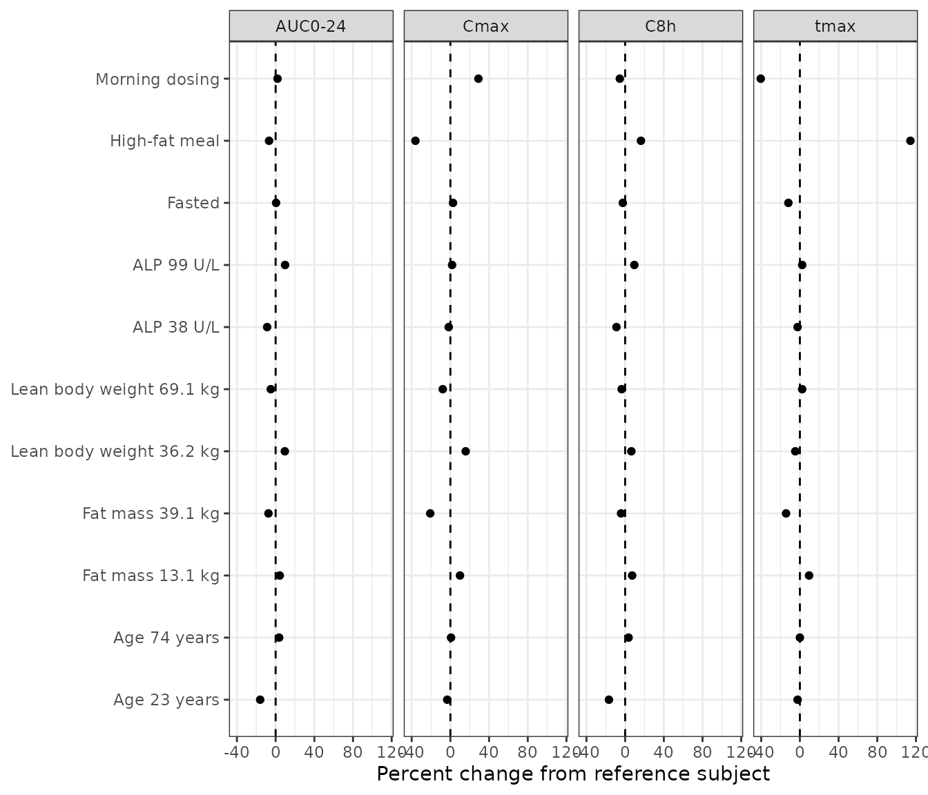
Replicates Figure 3b of Krause 2023: percent change of each exposure metric from the reference subject, one covariate at a time.
The food and dosing-time effects match the Results (high-fat meal: Cmax -36%, tmax 2.1 to 4.5 h; morning dosing: Cmax +29%, tmax 2.1 to 1.25 h). The paper states that all other covariates change exposure by less than 20%; the largest of them, Cmax at a fat mass of 39.1 kg, is -21% both here and in the published Figure 3a, so the statement is a rounded summary.
The tmax end points for lean body weight are not compared. The model gives 2.00 h at 36.2 kg and 2.15 h at 69.1 kg, a larger central volume delaying the peak; Figure 3a places the same two end points at about 2.00 h and 2.18 h but labels them the other way round, which would need the central volume to shrink with lean body weight, contrary to Table 2 and Table 3 and to the Cmax panel of the same figure.
Concentration-time profiles (Figure 4)
ev_fig4 <- dplyr::bind_rows(lapply(seq_along(scen_def), function(i) scen_events(i, names(scen_def)[i], n_days = 3)))
sim_fig4 <- rxode2::rxSolve(mod_typ, ev_fig4, keep = "scenario", returnType = "data.frame")
#> ℹ omega/sigma items treated as zero: 'etalfdepot', 'etaltlag', 'etalka', 'etalvc', 'etalvp', 'etalq', 'etalvmax', 'etalkm', 'etaiov_fdepot_1', 'etaiov_fdepot_2', 'etaiov_fdepot_3', 'etaiov_fdepot_4', 'etaiov_tlag_1', 'etaiov_tlag_2', 'etaiov_tlag_3', 'etaiov_tlag_4', 'etaiov_ka_1', 'etaiov_ka_2', 'etaiov_ka_3', 'etaiov_ka_4'
#> Warning: multi-subject simulation without without 'omega'
sim_fig4$scenario <- factor(sim_fig4$scenario, levels = names(scen_def))
ggplot2::ggplot(sim_fig4, ggplot2::aes(time, Cc, colour = scenario)) +
  ggplot2::geom_line() +
  ggplot2::labs(x = "Time (h)", y = "Daridorexant (ng/mL)", colour = NULL) +
  ggplot2::theme_bw()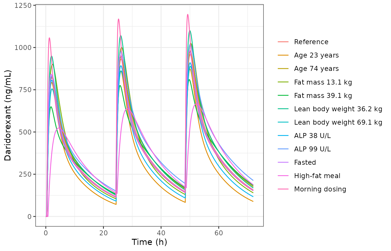
Replicates Figure 4 of Krause 2023: typical-value profiles with 50 mg once daily at bedtime for 3 days, one covariate varied at a time.
The reference-subject curve of Figure 4 (green, “Age: 60”) was digitised by the maintainers at times away from the steep absorption phase. The model follows it, including the modest rise of the trough over three days (from about 120 to 150 ng/mL) that the Michaelis-Menten elimination produces:
fig4_paper <- data.frame(
  time = c(8, 12, 16, 20, 23.5, 32, 40, 47.5, 56, 64, 71.5),
  paper = c(378, 274, 207, 157, 122, 462, 257, 152, 484, 270, 160)
)
ref4 <- sim_fig4[sim_fig4$scenario == "Reference", ]
fig4_paper$model <- stats::approx(ref4$time, ref4$Cc, xout = fig4_paper$time)$y
fig4_paper$pct_diff <- round(100 * (fig4_paper$model / fig4_paper$paper - 1), 1)
fig4_paper |>
  dplyr::mutate(model = signif(model, 4)) |>
  dplyr::rename(
    "Time (h)" = time, "Figure 4 (ng/mL)" = paper, "Model (ng/mL)" = model,
    "% diff" = pct_diff
  ) |>
knitr::kable(caption = "Reference-subject concentrations, 50 mg once daily at bedtime, model versus Figure 4.")| Time (h) | Figure 4 (ng/mL) | Model (ng/mL) | % diff |
|---|---|---|---|
| 8.0 | 378 | 382.2 | 1.1 |
| 12.0 | 274 | 276.9 | 1.1 |
| 16.0 | 207 | 209.4 | 1.2 |
| 20.0 | 157 | 159.0 | 1.2 |
| 23.5 | 122 | 124.7 | 2.2 |
| 32.0 | 462 | 465.1 | 0.7 |
| 40.0 | 257 | 259.6 | 1.0 |
| 47.5 | 152 | 155.2 | 2.1 |
| 56.0 | 484 | 485.6 | 0.3 |
| 64.0 | 270 | 272.1 | 0.8 |
| 71.5 | 160 | 162.9 | 1.8 |
Dose-dependent bioavailability and nonlinear elimination
Relative bioavailability follows
F = 0.41 * (DOSE / 50)^-0.47, so a 200 mg dose has 52% of
the bioavailability of a 50 mg dose (Results; Table 3). The apparent
clearance of the Michaelis-Menten term is Vm / (Km + C).
For the Table 2 reference values (Km = 2.36 ug/mL) it is 2.43 L/h at 500
ng/mL, the “2.4 L/h at concentrations of 500 ng/ml” of the
Discussion.
f_ratio <- (200 / 50)^-0.47
cl_500 <- 6.94 / (2.36 + 0.5)
c(F200_over_F50 = f_ratio, CL_at_500_ng_per_mL = cl_500)
#>       F200_over_F50 CL_at_500_ng_per_mL
#>           0.5212329           2.4265734
stopifnot(abs(f_ratio - 0.52) < 0.005, abs(cl_500 - 2.4) < 0.05)
doses <- c(5, 25, 50, 100, 200)
ev_dose <- dplyr::bind_rows(lapply(seq_along(doses), function(i) {
  scen_events(i, "Reference", dose = doses[i]) |> dplyr::mutate(scenario = paste(doses[i], "mg"))
}))
sim_dose <- rxode2::rxSolve(mod_typ, ev_dose, keep = "scenario", returnType = "data.frame")
#> ℹ omega/sigma items treated as zero: 'etalfdepot', 'etaltlag', 'etalka', 'etalvc', 'etalvp', 'etalq', 'etalvmax', 'etalkm', 'etaiov_fdepot_1', 'etaiov_fdepot_2', 'etaiov_fdepot_3', 'etaiov_fdepot_4', 'etaiov_tlag_1', 'etaiov_tlag_2', 'etaiov_tlag_3', 'etaiov_tlag_4', 'etaiov_ka_1', 'etaiov_ka_2', 'etaiov_ka_3', 'etaiov_ka_4'
#> Warning: multi-subject simulation without without 'omega'
sim_dose$scenario <- factor(sim_dose$scenario, levels = paste(doses, "mg"))
ggplot2::ggplot(sim_dose, ggplot2::aes(time, Cc, colour = scenario)) +
  ggplot2::geom_line() +
  ggplot2::labs(x = "Time after dose (h)", y = "Daridorexant (ng/mL)", colour = "Dose") +
  ggplot2::theme_bw()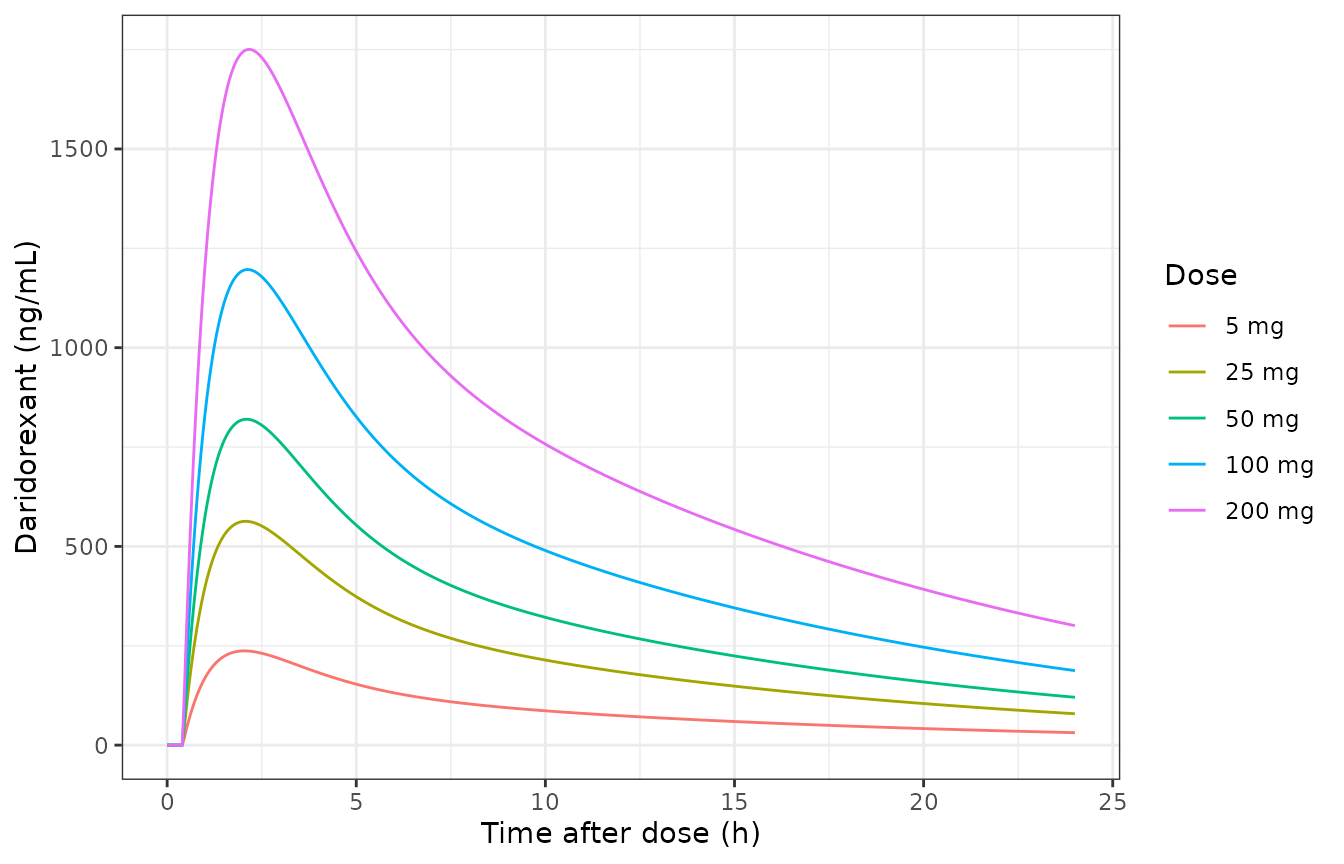
Typical-value single-dose profiles across the studied dose range (reference subject, bedtime, light meal).
Stochastic simulation in a virtual insomnia cohort
A virtual cohort of 200 patients receives 50 mg at bedtime with a light meal / uncontrolled food intake. Body composition is derived the way the paper did: lean body weight by the Janmahasatian formula from weight, BMI and sex, and fat mass as the difference between body weight and lean body weight. Weight, height, age and ALP distributions are chosen to land near the Table 1 medians; they are not taken from the paper.
rxode2::rxSetSeed(20230101)
n_sub <- 200
sexf <- stats::rbinom(n_sub, 1, 1155 / 1898)
ht_m <- ifelse(sexf == 1, stats::rnorm(n_sub, 1.63, 0.065), stats::rnorm(n_sub, 1.76, 0.07))
wt <- ifelse(sexf == 1, stats::rlnorm(n_sub, log(68), 0.17), stats::rlnorm(n_sub, log(80), 0.15))
wt <- pmin(pmax(wt, 42), 119.5)
bmi <- wt / ht_m^2
ffm <- ifelse(sexf == 1, 9270 * wt / (8780 + 244 * bmi), 9270 * wt / (6680 + 216 * bmi))
cohort <- data.frame(
  id = seq_len(n_sub),
  AGE = round(pmin(pmax(stats::rnorm(n_sub, 52, 16), 18), 88)),
  FFM = ffm,
  FM = wt - ffm,
  ALP = pmin(pmax(stats::rlnorm(n_sub, log(61), 0.3), 16), 244),
  DOSE = 50, FED = 1, FED_HIGHFAT = 0, DOSETIME_EVENING = 1, OCC = 1
)
summary(cohort[, c("AGE", "FFM", "FM", "ALP")])
#>       AGE             FFM              FM              ALP
#>  Min.   :18.00   Min.   :30.01   Min.   : 5.964   Min.   : 30.82
#>  1st Qu.:41.00   1st Qu.:40.47   1st Qu.:18.335   1st Qu.: 47.99
#>  Median :51.50   Median :45.74   Median :22.929   Median : 57.48
#>  Mean   :51.41   Mean   :49.17   Mean   :23.538   Mean   : 61.18
#>  3rd Qu.:62.00   3rd Qu.:56.74   3rd Qu.:28.537   3rd Qu.: 70.03
#>  Max.   :88.00   Max.   :75.66   Max.   :56.742   Max.   :155.03
obs_grid <- data.frame(time = c(0, 0.25, 0.5, 0.75, 1, 1.5, 2, 2.5, 3, 4, 5, 6, 8, 9, 10, 12, 16, 20, 24))
ev_st <- dplyr::bind_rows(
  dplyr::mutate(cohort, time = 0, amt = 50, evid = 1L, cmt = "depot"),
  dplyr::cross_join(cohort, obs_grid) |> dplyr::mutate(amt = 0, evid = 0L, cmt = "central")
) |>
  dplyr::arrange(id, time, dplyr::desc(evid)) |>
  # Event columns first: rxode2 reads a DOSE column that precedes amt as the
  # dose amount rather than as a covariate.
  dplyr::select(id, time, amt, evid, cmt, dplyr::everything())
sim_st <- rxode2::rxSolve(mod, ev_st, returnType = "data.frame")
#> ℹ parameter labels from comments will be replaced by 'label()'
#> Warning: some etas defaulted to non-mu referenced, possible parsing error: etaiov_fdepot_1, etaiov_fdepot_2, etaiov_fdepot_3, etaiov_fdepot_4, etaiov_tlag_1, etaiov_tlag_2, etaiov_tlag_3, etaiov_tlag_4, etaiov_ka_1, etaiov_ka_2, etaiov_ka_3, etaiov_ka_4
#> as a work-around try putting the mu-referenced expression on a simple line
sim_st$treatment <- "50 mg bedtime"
sim_st |>
  dplyr::group_by(time) |>
  dplyr::summarise(
    p05 = stats::quantile(sim, 0.05), p50 = stats::median(sim), p95 = stats::quantile(sim, 0.95),
    .groups = "drop"
  ) |>
  ggplot2::ggplot(ggplot2::aes(time, p50)) +
  ggplot2::geom_ribbon(ggplot2::aes(ymin = p05, ymax = p95), alpha = 0.25) +
  ggplot2::geom_line() +
  ggplot2::labs(x = "Time after dose (h)", y = "Daridorexant (ng/mL)") +
  ggplot2::theme_bw()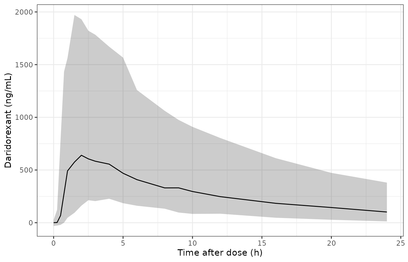
Stochastic simulation, 50 mg at bedtime: median and 5th-95th percentiles of plasma daridorexant (residual error included).
PKNCA on the individual predictions (Cc, without
residual error):
conc_st <- PKNCA::PKNCAconc(
  dplyr::filter(sim_st, !is.na(Cc)),
  Cc ~ time | treatment + id
)
dose_st <- PKNCA::PKNCAdose(
  dplyr::filter(ev_st, evid == 1) |> dplyr::mutate(treatment = "50 mg bedtime"),
  amt ~ time | treatment + id
)
nca_st <- PKNCA::pk.nca(PKNCA::PKNCAdata(conc_st, dose_st, intervals = intervals))
summary(nca_st)
#>  start end     treatment   N     auclast       cmax               tmax
#>      0  24 50 mg bedtime 200 7280 [64.6] 727 [69.2] 2.00 [0.750, 10.0]
#>
#> Caption: auclast, cmax: geometric mean and geometric coefficient of variation; tmax: median and range; N: number of subjects

st_res <- as.data.frame(nca_st$result)
med_cmax <- stats::median(st_res$PPORRES[st_res$PPTESTCD == "cmax"])
med_auc <- stats::median(st_res$PPORRES[st_res$PPTESTCD == "auclast"])
c(median_cmax = med_cmax, median_auclast = med_auc)
#>    median_cmax median_auclast
#>       744.7668      7192.3775
stopifnot(
  # The cohort median sits near the typical-value reference subject; the
  # cohort's own covariate mix and the log-normal IIV on F shift it by at most
  # tens of percent, while a unit or structural error would shift it by far more.
  abs(log(med_cmax / ref_row$cmax)) < log(1.3),
  abs(log(med_auc / ref_row$auclast)) < log(1.3)
)
Assumptions and deviations
- Age reference. The Table 2 footnote gives an age reference of 30 years, while the Figure 3 “typical subject” is 60 years old. The model uses the footnote’s 30 years: with it the reference subject’s simulated AUC0-24, Cmax, C8h and tmax match Figure 3a and the Results to within 1%, whereas a 60-year reference lowers AUC0-24 by about 12% and C8h by about 12%.
-
Residual error form. The paper reports an additive
(17.59 ng/mL) and a multiplicative (0.16) error term but does not name
the Monolix error model. The Monolix default combined form
combined1,y = f + (a + b*f)*e, is used. - Units of the additive error. Not printed; ng/mL is used, the unit of the paper’s concentrations (Km is printed in ug/mL and is converted inside the model, where the central concentration is in mg/L).
-
Inter-occasion variability. Table 2 reports one IOV
SD each for F, tlag and ka but not how occasions were defined. The model
carries four occasion slots (
OCC= 1-4) with equal variances; records withOCCoutside 1-4 get no IOV. The simulations above useOCC = 1. -
Food status encoding. The paper’s three-level food
status (fasted, light meal / uncontrolled, high-fat high-calorie meal;
reference light meal / uncontrolled) is carried by the existing
FEDandFED_HIGHFATindicators: fasted isFED = 0, the reference isFED = 1, FED_HIGHFAT = 0, and a high-fat meal isFED = 1, FED_HIGHFAT = 1. -
Dosing time. Bedtime administration is the
reference (
DOSETIME_EVENING = 1); morning dosing (DOSETIME_EVENING = 0) multiplies ka by exp(1.05). -
Lean body weight. The paper’s “lean body weight” is
computed with the Janmahasatian formula, which the covariate register
files under
FFM. - Distribution of F. Table 2 states that all parameters are log-normally distributed, so F carries a log-normal IIV and IOV as printed; a sampled individual F above 1 is possible for large positive random effects. F is a relative bioavailability, so this is not a contradiction in the model.
- Errata in the Discussion. The Discussion states “t lag 0.41 and 1.23 h, k a 3.8 and 1.05/h in the fasted and fed states”. These values do not follow from Table 2, whose own footnote derives tlag = 0.25 h (fasted) and 0.76 h (fed), matching the Results (15, 25 and 46 min) and the Table 3 ratios (tlag fed / fasted = 3.1, ka fasted / fed = 3.6). The model follows Table 2. Likewise the Discussion’s “1.8 L/h at 1000 ng/mL” does not follow from the Table 2 reference Km (which gives 2.07 L/h); it matches a 60-year-old subject (Km 2.90 ug/mL). The Table 2 values are used unchanged.
- Figure 3a lean-body-weight tmax labels. Figure 3a labels the two lean-body-weight tmax end points the opposite way round from what a central volume that grows with lean body weight (Table 2, Table 3, and the Cmax panel of the same figure) implies. The magnitudes agree with the model; the direction is taken from the parameter table, and these two end points are left out of the Figure 3 comparison.
- Virtual cohort. Weight, height, age and ALP distributions are chosen by the maintainers to land near the Table 1 medians; the paper does not give joint distributions.