Lecanemab PK, amyloid PET SUVr and plasma biomarkers (Hayato 2022)
Source:vignettes/articles/Hayato_2022_lecanemab.Rmd
Hayato_2022_lecanemab.RmdModel and source
Hayato 2022 reports one population PK model for intravenous lecanemab and three PK/PD models fitted sequentially on its post hoc individual PK parameters. Following the authors’ structure, the library carries four models:
| Model | Endpoint |
|---|---|
Hayato_2022_lecanemab |
Serum lecanemab (two-compartment PK) |
Hayato_2022_lecanemab_suvr |
Amyloid PET SUVr (indirect response, Emax stimulation of loss) |
Hayato_2022_lecanemab_abeta4240 |
Plasma Abeta42/40 ratio (indirect response, linear stimulation of production) |
Hayato_2022_lecanemab_ptau181 |
Plasma p-tau181 (indirect response, linear inhibition of production) |
Each PK/PD model embeds the PK model with its parameters and IIV fixed, so it can be simulated from a dosing record alone.
mod_names <- c(
  pk = "Hayato_2022_lecanemab",
  suvr = "Hayato_2022_lecanemab_suvr",
  abeta4240 = "Hayato_2022_lecanemab_abeta4240",
  ptau181 = "Hayato_2022_lecanemab_ptau181"
)
mods <- lapply(mod_names, function(nm) rxode2::rxode(readModelDb(nm)))
#> ℹ parameter labels from comments will be replaced by 'label()'
#> ℹ parameter labels from comments will be replaced by 'label()'
#> ℹ parameter labels from comments will be replaced by 'label()'
#> ℹ parameter labels from comments will be replaced by 'label()'- Citation: Hayato S, Takenaka O, Sreerama Reddy SH, Landry I, Reyderman L, Koyama A, Swanson C, Yasuda S, Hussein Z (2022). Population pharmacokinetic-pharmacodynamic analyses of amyloid positron emission tomography and plasma biomarkers for lecanemab in subjects with early Alzheimer’s disease. CPT Pharmacometrics Syst Pharmacol 11(12):1578-1591. doi:10.1002/psp4.12862.
- Article: https://doi.org/10.1002/psp4.12862 (open access; supplementary Texts S1-S4 hold the four NONMEM control streams)
Population
The PK dataset holds 9027 serum lecanemab concentrations from 725 subjects in the phase 1 studies 101 (single and multiple ascending doses, mild-to-moderate Alzheimer’s disease) and 104 (multiple ascending doses, MCI due to AD or mild AD) and the phase 2 study 201 (Core: placebo, 2.5 mg/kg biweekly, 5 mg/kg monthly or biweekly, 10 mg/kg monthly or biweekly for 18 months; then a 9-59 month off-treatment gap and an open-label extension at 10 mg/kg biweekly). Supplement Table S2 gives the PK population as mean age 71.0 years (50-93), mean weight 73.7 kg (41.2-124.7), mean albumin 42.9 g/L, 46.9% female, 86.3% White and 6.9% Japanese. The PK/PD datasets are from study 201 only: 374 subjects / 1213 SUVr measurements, 284 subjects / 1254 plasma Abeta42/40 ratios, and 562 subjects / 2021 plasma p-tau181 values, with about 70% APOE4 carriers and about two-thirds MCI due to AD in each.
The same information is available programmatically, e.g.
readModelDb("Hayato_2022_lecanemab_suvr")()$population.
Source trace
Every ini() value carries an in-file comment pointing to
its source. All estimates are the final NONMEM estimates of Tables 1-3;
the functional forms come from the equations printed under those tables
and from the supplementary control streams (Model S1 = PK, S2 = SUVr, S3
= Abeta42/40, S4 = p-tau181).
| Parameter | Value | Source |
|---|---|---|
| CL, V1, Q, V2 | 0.0181 L/h, 3.22 L, 0.0349 L/h, 2.19 L | Table 1 |
| F for Process B (Process A fixed 1) | 0.998 | Table 1; Model S1
F1=1; IF (FORM.EQ.1) F1=THETA(11)*EXP(ETA(4))
|
| WT on CL / V1 (power, 73.7 kg) | 0.403 / 0.606 | Table 1 and equations; Model S1 (WGT/73.7)
|
| ALB on CL (power, 42.9 g/L) | -0.243 | Table 1 and equation |
| Female on CL / V1 (ratio) | 0.792 / 0.893 | Table 1 |
| ADA-positive on CL (ratio) | 1.09 | Table 1 |
| Japanese on V2 (ratio) | 0.455 | Table 1 |
| IIV CL, V1, V2, F (CV% = 100 x SD) | 38.9, 14.0, 99.5, 34.2 | Table 1 |
| Proportional RUV study 101 / 104 / 201 | 14.0%, 19.7%, 30.3% | Table 1; Model S1 $ERROR
(W = F + 0.01) |
| SUVr baseline, Kin | 1.34, 0.232 SUVr/year | Table 2; Model S2 KIN = THETA(2)/8760,
KOUT = KIN/BSL
|
| SUVr Emax, EC50 | 1.54, 75.0 ug/mL | Table 2 |
| APOE4 carrier on SUVr baseline (ratio) | 1.04 | Table 2 |
| Age on Emax (power, 72 years) | 1.58 | Table 2; Model S2 (AGE/72)**THETA(5)
|
| IIV SUVr baseline, Emax; correlation | 10.9%, 50.3%; R = 0.669 | Table 2; Model S2 $OMEGA BLOCK(2)
|
| SUVr proportional RUV | 5.01% | Table 2 |
| Abeta42/40 baseline, Kout, slope | 0.0842, 0.367 /year, 0.00155 per ug/mL | Table 3 |
| IIV Abeta42/40 baseline, slope | 6.78%, 44.1% | Table 3 |
| Abeta42/40 proportional RUV | 6.41% | Table 3; Model S3 W = IPRED*THETA(4),
$SIGMA 1 FIX
|
| p-tau181 baseline, Kout, slope | 4.06 pg/mL, 0.468 /year, 0.00313 per ug/mL | Table 3 |
| WT on p-tau181 baseline (power, 72.2 kg) | -0.300 | Table 3; Model S4 (BWGTC/72.2)**THETA(5)
|
| IIV p-tau181 baseline (exponential), slope (additive SD) | 35.1%, 0.00151 per ug/mL | Table 3; Model S4 SLOPE = THETA(3)+ETA(2)
|
| p-tau181 proportional RUV | 19.4% | Table 3 |
| PK ODEs | n/a | Figure 1; Model S1 ADVAN3 TRANS4
|
d/dt(suvr) = kin - suvr * kout * (1 + emax * Cc / (ec50 + Cc)) |
n/a | Figure 1; Model S2 $DES
|
d/dt(abeta4240) = kin * (1 + slope * Cc) - kout * abeta4240 |
n/a | Figure 1; Model S3 $DES
|
d/dt(ptau181) = kin * (1 - slope * (Cc + 0.01)) - kout * ptau181 |
n/a | Figure 1; Model S4 $DES
|
Event-table helpers
Doses are 10 mg/kg intravenous infusions over 1 hour into
central. The reference subject of the Figure 2 forest plot
is a 73.7 kg non-Japanese male, albumin 42.9 g/L, ADA-negative, dosed
with Process A material; the PD reference subject is 72 years old and an
APOE4 non-carrier.
h_per_year <- 8760
h_per_month <- h_per_year / 12

ref_cov <- list(
  WT = 73.7, ALB = 42.9, SEXF = 0, ADA_POS = 0, RACE_JAPANESE = 0,
  FORM_LEC_PROCESSB = 0, STUDY_LEC101 = 0, STUDY_LEC104 = 0,
  AGE = 72, APOE4_CARRIER = 0
)

# One subject: 10 mg/kg infusions every `tau` hours from time 0 until
# `dose_end` (exclusive), observations on the ODE state `obs_cmt`.
make_subject <- function(id, tau, dose_end, obs_times, obs_cmt = "central",
                         label = NA_character_, cov = list()) {
  covs <- utils::modifyList(ref_cov, cov)
  dose_times <- if (dose_end > 0) seq(0, dose_end - 1e-6, by = tau) else numeric(0)
  amt <- 10 * covs$WT
  doses <- if (length(dose_times) > 0) {
    data.frame(
      id = id, time = dose_times, evid = 1L, amt = amt, rate = amt,
      cmt = "central"
    )
  }
  obs <- data.frame(
    id = id, time = sort(unique(obs_times)), evid = 0L, amt = 0, rate = 0,
    cmt = obs_cmt
  )
  ev <- dplyr::bind_rows(doses, obs) |>
    dplyr::arrange(time, dplyr::desc(evid))
  for (nm in names(covs)) ev[[nm]] <- covs[[nm]]
  ev$scenario <- label
  ev
}
PK model
Terminal half-life
The Discussion gives a typical terminal half-life of about 9.5 days. The closed form from the Table 1 micro-constants:
k10 <- 0.0181 / 3.22
k12 <- 0.0349 / 3.22
k21 <- 0.0349 / 2.19
beta <- 0.5 * (k10 + k12 + k21 - sqrt((k10 + k12 + k21)^2 - 4 * k10 * k21))
t_half_days <- log(2) / beta / 24
t_half_days
#> [1] 9.460475
stopifnot(abs(t_half_days - 9.5) < 0.1)
The same quantity estimated by PKNCA from a simulated single 10 mg/kg dose in the reference subject:
sd_times <- c(0, 0.5, 1, 1.5, 2, 4, 8, 24, 48, 96, 168, 336, 504, 672,
              1008, 1344, 1680, 2016)
ev_sd <- make_subject(1L, tau = 1e6, dose_end = 1, obs_times = sd_times,
                      label = "10 mg/kg single dose")
sim_sd <- rxode2::rxSolve(rxode2::zeroRe(mods$pk), ev_sd, keep = "scenario",
                          returnType = "data.frame")
#> Warning: No sigma parameters in the model
#> ℹ omega/sigma items treated as zero: 'etalcl', 'etalvc', 'etalvp', 'etalfcentral'
if (is.null(sim_sd$id)) sim_sd$id <- 1L

conc_sd <- sim_sd |>
  dplyr::filter(!is.na(Cc)) |>
  dplyr::select(id, time, Cc, scenario)
dose_sd <- ev_sd |>
  dplyr::filter(evid == 1) |>
  dplyr::select(id, time, amt, scenario)
nca_sd <- PKNCA::pk.nca(PKNCA::PKNCAdata(
  PKNCA::PKNCAconc(conc_sd, Cc ~ time | scenario + id),
  PKNCA::PKNCAdose(dose_sd, amt ~ time | scenario + id),
  intervals = data.frame(start = 0, end = Inf, cmax = TRUE, half.life = TRUE)
))

published_sd <- data.frame(scenario = "10 mg/kg single dose", half.life = 9.5 * 24)
cmp_sd <- nlmixr2lib::ncaComparisonTable(
  simulated = nca_sd,
  reference = published_sd,
  by = "scenario",
  params = "half.life",
  units = c(half.life = "h")
)
knitr::kable(cmp_sd, caption = "Typical terminal half-life: simulated vs the Discussion's ~9.5 days.")| NCA parameter | scenario | Reference | Simulated | % diff |
|---|---|---|---|---|
| t½ (h) | 10 mg/kg single dose | 228 | 227 | -0.5% |
Steady-state covariate effects (Figure 2)
Figure 2 shows steady-state AUC and Cmax after 10 mg/kg biweekly for the 5th and 95th percentiles of weight and albumin and for each binary covariate, relative to the reference subject. The typical-value model is simulated for one year (26 doses) and PKNCA computes Cmax and AUC over the last dosing interval. Because the dose is weight-based, the weight rows combine the dose change with the CL and V1 effects.
scenarios <- list(
  "Reference" = list(),
  "Weight 51 kg" = list(WT = 51),
  "Weight 99 kg" = list(WT = 99),
  "Albumin 38 g/L" = list(ALB = 38),
  "Albumin 48 g/L" = list(ALB = 48),
  "Female" = list(SEXF = 1),
  "Japanese" = list(RACE_JAPANESE = 1),
  "Process B" = list(FORM_LEC_PROCESSB = 1),
  "ADA-positive" = list(ADA_POS = 1)
)
tau <- 14 * 24
t_last <- 25 * tau
ss_times <- t_last + c(0, 0.5, 1, 1.5, 2, 4, 8, 12, 24, 48, 96, 168, 240, 336)
ev_ss <- dplyr::bind_rows(lapply(seq_along(scenarios), function(i) {
  make_subject(i, tau = tau, dose_end = t_last + 1, obs_times = ss_times,
               label = names(scenarios)[i], cov = scenarios[[i]])
}))
stopifnot(!anyDuplicated(unique(ev_ss[, c("id", "time", "evid")])))

sim_ss <- rxode2::rxSolve(rxode2::zeroRe(mods$pk), ev_ss, keep = "scenario",
                          returnType = "data.frame")
#> Warning: No sigma parameters in the model
#> ℹ omega/sigma items treated as zero: 'etalcl', 'etalvc', 'etalvp', 'etalfcentral'
#> Warning: multi-subject simulation without without 'omega'

conc_ss <- sim_ss |>
  dplyr::filter(!is.na(Cc)) |>
  dplyr::select(id, time, Cc, scenario)
dose_ss <- ev_ss |>
  dplyr::filter(evid == 1) |>
  dplyr::select(id, time, amt, scenario)
nca_ss <- PKNCA::pk.nca(PKNCA::PKNCAdata(
  PKNCA::PKNCAconc(conc_ss, Cc ~ time | scenario + id),
  PKNCA::PKNCAdose(dose_ss, amt ~ time | scenario + id),
  intervals = data.frame(start = t_last, end = t_last + tau,
                         cmax = TRUE, auclast = TRUE)
))
ss_wide <- as.data.frame(nca_ss) |>
  dplyr::filter(PPTESTCD %in% c("cmax", "auclast")) |>
  dplyr::select(scenario, PPTESTCD, PPORRES) |>
  tidyr::pivot_wider(names_from = PPTESTCD, values_from = PPORRES)
ref_row <- ss_wide[ss_wide$scenario == "Reference", ]
ss_ratio <- ss_wide |>
  dplyr::mutate(auclast = auclast / ref_row$auclast, cmax = cmax / ref_row$cmax)
knitr::kable(
  ss_wide |>
    dplyr::rename("Scenario" = scenario, "AUCtau (ug*h/mL)" = auclast, "Cmax (ug/mL)" = cmax),
  digits = 1,
  caption = "Typical steady-state exposure after 10 mg/kg biweekly (last interval of 26 doses)."
)| Scenario | AUCtau (ug*h/mL) | Cmax (ug/mL) |
|---|---|---|
| ADA-positive | 37536.9 | 281.1 |
| Albumin 38 g/L | 39717.7 | 286.6 |
| Albumin 48 g/L | 42028.3 | 292.5 |
| Female | 51628.2 | 341.5 |
| Japanese | 40802.7 | 280.6 |
| Process B | 40819.0 | 289.0 |
| Reference | 40900.9 | 289.6 |
| Weight 51 kg | 32852.2 | 246.8 |
| Weight 99 kg | 48754.5 | 329.8 |
The AUC ratio has a closed form, dose ratio x F / CL ratio, against which the PKNCA ratios are checked tightly; the Figure 2 medians were read off the published plot by the maintainers (reading precision about +/- 0.02).
closed_form_auc <- c(
  "Reference" = 1,
  "Weight 51 kg" = (51 / 73.7)^(1 - 0.403),
  "Weight 99 kg" = (99 / 73.7)^(1 - 0.403),
  "Albumin 38 g/L" = (38 / 42.9)^0.243,
  "Albumin 48 g/L" = (48 / 42.9)^0.243,
  "Female" = 1 / 0.792,
  "Japanese" = 1,
  "Process B" = 0.998,
  "ADA-positive" = 1 / 1.09
)
stopifnot(all(abs(ss_ratio$auclast - closed_form_auc[ss_ratio$scenario]) < 0.005))

# Medians digitised from Figure 2 (circle = AUC, triangle = Cmax).
figure2 <- data.frame(
  scenario = names(scenarios),
  auclast = c(1.00, 0.805, 1.20, 0.97, 1.025, 1.265, 1.00, 1.00, 0.915),
  cmax = c(1.00, 0.855, 1.14, 0.99, 1.01, 1.18, 0.97, 0.995, 0.97)
)
cmp_forest <- nlmixr2lib::ncaComparisonTable(
  simulated = ss_ratio,
  reference = figure2,
  by = "scenario",
  units = c(auclast = "ratio to reference", cmax = "ratio to reference"),
  tolerance_pct = 5
)
knitr::kable(cmp_forest, caption = "Steady-state AUCtau and Cmax relative to the reference subject: simulated vs Figure 2 (digitised medians). * differs by > 5%.")| NCA parameter | scenario | Reference | Simulated | % diff |
|---|---|---|---|---|
| Cmax (ratio to reference) | Reference | 1 | 1 | +0.0% |
| Cmax (ratio to reference) | Weight 51 kg | 0.855 | 0.852 | -0.3% |
| Cmax (ratio to reference) | Weight 99 kg | 1.14 | 1.14 | -0.1% |
| Cmax (ratio to reference) | Albumin 38 g/L | 0.99 | 0.99 | -0.0% |
| Cmax (ratio to reference) | Albumin 48 g/L | 1.01 | 1.01 | +0.0% |
| Cmax (ratio to reference) | Female | 1.18 | 1.18 | -0.1% |
| Cmax (ratio to reference) | Japanese | 0.97 | 0.969 | -0.1% |
| Cmax (ratio to reference) | Process B | 0.995 | 0.998 | +0.3% |
| Cmax (ratio to reference) | ADA-positive | 0.97 | 0.97 | +0.1% |
| AUClast (ratio to reference) | Reference | 1 | 1 | +0.0% |
| AUClast (ratio to reference) | Weight 51 kg | 0.805 | 0.803 | -0.2% |
| AUClast (ratio to reference) | Weight 99 kg | 1.2 | 1.19 | -0.7% |
| AUClast (ratio to reference) | Albumin 38 g/L | 0.97 | 0.971 | +0.1% |
| AUClast (ratio to reference) | Albumin 48 g/L | 1.02 | 1.03 | +0.3% |
| AUClast (ratio to reference) | Female | 1.26 | 1.26 | -0.2% |
| AUClast (ratio to reference) | Japanese | 1 | 0.998 | -0.2% |
| AUClast (ratio to reference) | Process B | 1 | 0.998 | -0.2% |
| AUClast (ratio to reference) | ADA-positive | 0.915 | 0.918 | +0.3% |
Amyloid PET SUVr model
Re-accumulation half-life
Kout = Kin / baseline = 0.232 / 1.34 = 0.173 per year, the value quoted in the Discussion, so the recovery half-life after treatment stops is about 4 years:
Typical profiles (Figures 4 and 5)
Figure 4 compares 10 mg/kg biweekly with 10 mg/kg monthly for 18 months, with the baseline SUVr set to 1.38 (the study 201 median). Figure 5 continues 10 mg/kg biweekly for 15 years or stops it at 18 months. The same four regimens are simulated for all three biomarkers from the typical-value models; the SUVr baseline is overridden to 1.38 as in the figures.
t18 <- 18 * h_per_month
t15y <- 15 * h_per_year
obs_typ <- sort(unique(c(seq(0, t15y, by = 14 * 24), t18, t15y)))
regimens <- list(
  "10 mg/kg biweekly, 18 months" = list(tau = 14 * 24, dose_end = t18),
  "10 mg/kg monthly, 18 months" = list(tau = 28 * 24, dose_end = t18),
  "10 mg/kg biweekly, continuous" = list(tau = 14 * 24, dose_end = t15y)
)
sim_typical <- function(endpoint, ui) {
  ev <- dplyr::bind_rows(lapply(seq_along(regimens), function(i) {
    make_subject(i, tau = regimens[[i]]$tau, dose_end = regimens[[i]]$dose_end,
                 obs_times = obs_typ, obs_cmt = endpoint, label = names(regimens)[i])
  }))
  sim <- rxode2::rxSolve(rxode2::zeroRe(ui), ev, keep = "scenario",
                         returnType = "data.frame")
  data.frame(endpoint = endpoint, scenario = sim$scenario, time = sim$time,
             value = sim[[endpoint]])
}
typ <- dplyr::bind_rows(
  sim_typical("suvr", rxode2::ini(mods$suvr, lrbase = log(1.38))),
  sim_typical("abeta4240", mods$abeta4240),
  sim_typical("ptau181", mods$ptau181)
)
#> ℹ change initial estimate of `lrbase` to `0.322083499169113`
#> ℹ omega/sigma items treated as zero: 'etalcl', 'etalvc', 'etalvp', 'etalfcentral', 'etalrbase', 'etalemax'
#> Warning: multi-subject simulation without without 'omega'
#> ℹ omega/sigma items treated as zero: 'etalcl', 'etalvc', 'etalvp', 'etalfcentral', 'etalrbase', 'etalslope'
#> Warning: multi-subject simulation without without 'omega'
#> ℹ omega/sigma items treated as zero: 'etalcl', 'etalvc', 'etalvp', 'etalfcentral', 'etalrbase', 'etaslope'
#> Warning: multi-subject simulation without without 'omega'
typ |>
  dplyr::filter(time <= t18, scenario != "10 mg/kg biweekly, continuous") |>
  ggplot(aes(time / h_per_month, value, colour = scenario)) +
  geom_line() +
  geom_hline(data = data.frame(endpoint = "suvr", y = 1.17),
             aes(yintercept = y), linetype = "dashed") +
  facet_wrap(~endpoint, scales = "free_y") +
  labs(x = "Time (months)", y = NULL, colour = NULL,
       caption = "Replicates Figure 4 of Hayato 2022 (typical values; dashed line: SUVr 1.17).") +
  theme(legend.position = "bottom")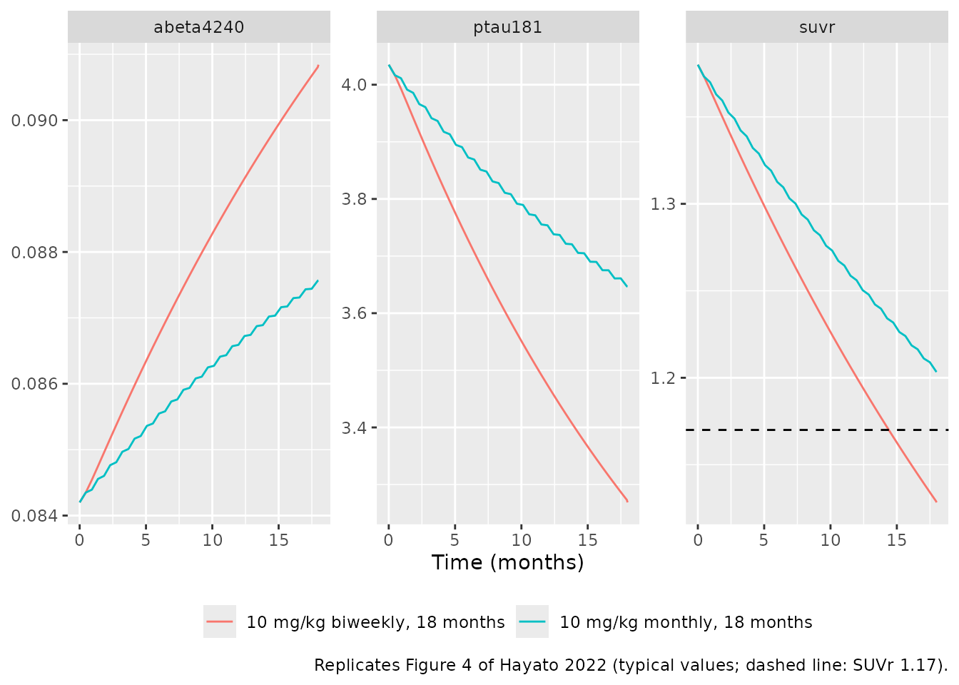
typ |>
  dplyr::filter(scenario != "10 mg/kg monthly, 18 months") |>
  ggplot(aes(time / h_per_year, value, colour = scenario)) +
  geom_line() +
  geom_vline(xintercept = 1.5, linetype = "dotted") +
  facet_wrap(~endpoint, scales = "free_y") +
  labs(x = "Time (years)", y = NULL, colour = NULL,
       caption = "Replicates Figure 5 of Hayato 2022 (typical values).") +
  theme(legend.position = "bottom")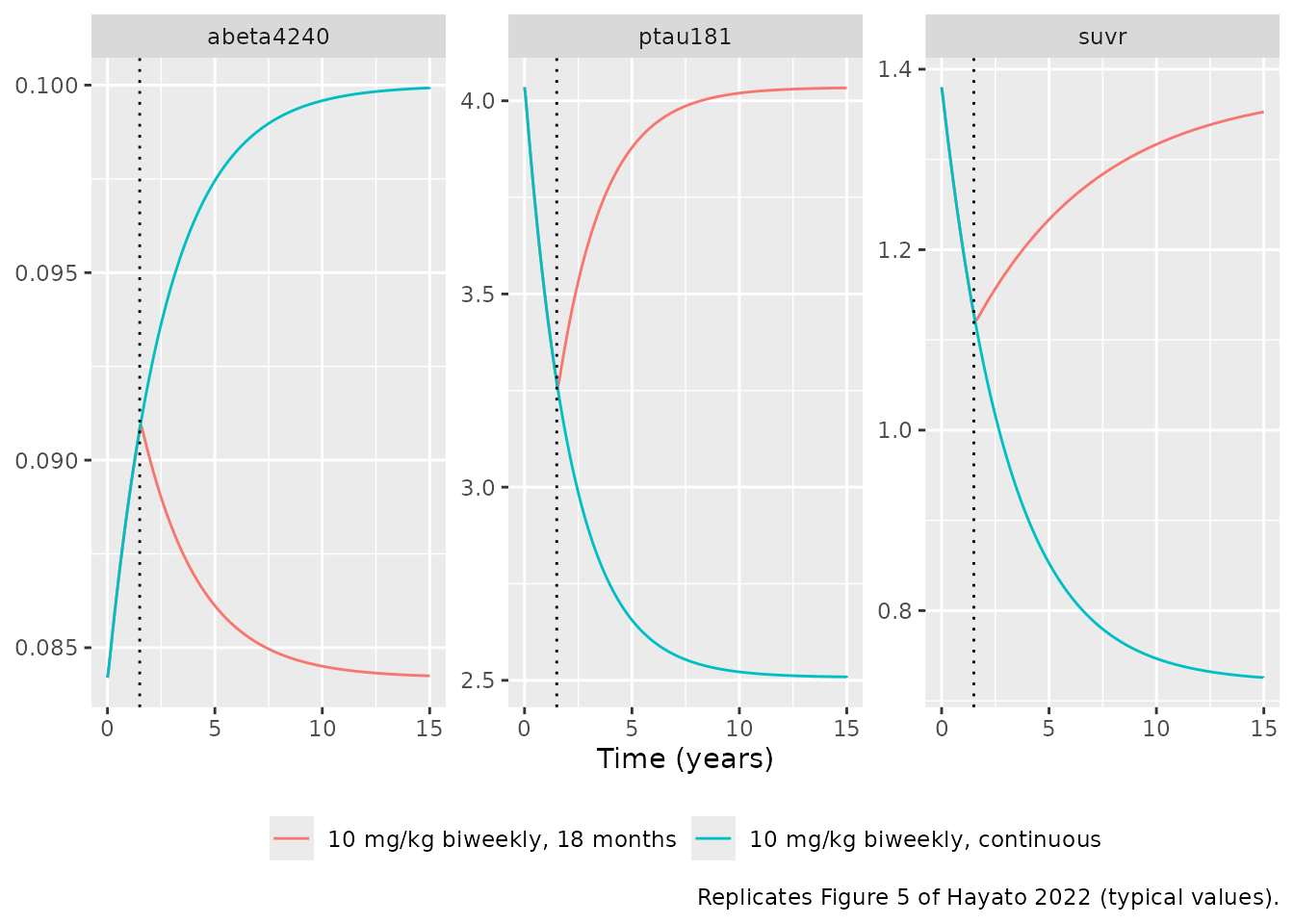
The values at 18 months and at 15 years, against values read off Figures 4 and 5 by the maintainers. The published curves are medians over 1000 draws of the PD parameter uncertainty, so a close but not exact match is expected.
pick <- function(ep, sc, t) {
  v <- typ$value[typ$endpoint == ep & typ$scenario == sc & abs(typ$time - t) < 1e-6]
  if (length(v) != 1L) stop("no unique row for ", ep, " / ", sc, " at ", t)
  v
}
checks <- tibble::tribble(
  ~endpoint, ~scenario, ~time_h, ~figure, ~published,
  "suvr", "10 mg/kg biweekly, 18 months", t18, "Figure 4", 1.14,
  "suvr", "10 mg/kg monthly, 18 months", t18, "Figure 4", 1.215,
  "abeta4240", "10 mg/kg biweekly, 18 months", t18, "Figure 4", 0.0904,
  "abeta4240", "10 mg/kg monthly, 18 months", t18, "Figure 4", 0.0873,
  "ptau181", "10 mg/kg biweekly, 18 months", t18, "Figure 4", 3.33,
  "ptau181", "10 mg/kg monthly, 18 months", t18, "Figure 4", 3.68,
  "suvr", "10 mg/kg biweekly, continuous", t15y, "Figure 5", 0.725,
  "suvr", "10 mg/kg biweekly, 18 months", t15y, "Figure 5", 1.355,
  "abeta4240", "10 mg/kg biweekly, continuous", t15y, "Figure 5", 0.0987,
  "ptau181", "10 mg/kg biweekly, continuous", t15y, "Figure 5", 2.62
)
checks$simulated <- mapply(pick, checks$endpoint, checks$scenario, checks$time_h)
checks$pct_diff <- 100 * (checks$simulated / checks$published - 1)
checks |>
  dplyr::mutate(time = ifelse(time_h == t18, "18 months", "15 years")) |>
  dplyr::select(figure, endpoint, scenario, time, published, simulated, pct_diff) |>
  dplyr::rename("Figure" = figure, "Endpoint" = endpoint, "Regimen" = scenario,
                "Time" = time, "Published (digitised)" = published,
                "Simulated" = simulated, "% diff" = pct_diff) |>
  knitr::kable(digits = c(0, 0, 0, 0, 4, 4, 1),
caption = "Typical biomarker values: simulated vs Figures 4 and 5.")| Figure | Endpoint | Regimen | Time | Published (digitised) | Simulated | % diff |
|---|---|---|---|---|---|---|
| Figure 4 | suvr | 10 mg/kg biweekly, 18 months | 18 months | 1.1400 | 1.1283 | -1.0 |
| Figure 4 | suvr | 10 mg/kg monthly, 18 months | 18 months | 1.2150 | 1.2034 | -1.0 |
| Figure 4 | abeta4240 | 10 mg/kg biweekly, 18 months | 18 months | 0.0904 | 0.0908 | 0.5 |
| Figure 4 | abeta4240 | 10 mg/kg monthly, 18 months | 18 months | 0.0873 | 0.0876 | 0.3 |
| Figure 4 | ptau181 | 10 mg/kg biweekly, 18 months | 18 months | 3.3300 | 3.2688 | -1.8 |
| Figure 4 | ptau181 | 10 mg/kg monthly, 18 months | 18 months | 3.6800 | 3.6467 | -0.9 |
| Figure 5 | suvr | 10 mg/kg biweekly, continuous | 15 years | 0.7250 | 0.7257 | 0.1 |
| Figure 5 | suvr | 10 mg/kg biweekly, 18 months | 15 years | 1.3550 | 1.3527 | -0.2 |
| Figure 5 | abeta4240 | 10 mg/kg biweekly, continuous | 15 years | 0.0987 | 0.0999 | 1.3 |
| Figure 5 | ptau181 | 10 mg/kg biweekly, continuous | 15 years | 2.6200 | 2.5068 | -4.3 |
The largest difference is the p-tau181 plateau under 15 years of continuous dosing (about 4% below the figure); the 18-month values, which the trial data inform directly, agree within 2%.
Age effect on the SUVr reduction (Figure S5)
The Results state that, after 18 months of 10 mg/kg biweekly, an 84-year-old has a 24% larger and a 57-year-old a 29% smaller SUVr reduction than a 72-year-old reference APOE4 non-carrier.
ages <- c(72, 84, 57)
ev_age <- dplyr::bind_rows(lapply(seq_along(ages), function(i) {
  make_subject(i, tau = 14 * 24, dose_end = t18, obs_times = c(0, t18),
               obs_cmt = "suvr", label = paste0("Age ", ages[i]),
               cov = list(AGE = ages[i]))
}))
sim_age <- rxode2::rxSolve(rxode2::zeroRe(mods$suvr), ev_age, keep = "scenario",
                           returnType = "data.frame")
#> ℹ omega/sigma items treated as zero: 'etalcl', 'etalvc', 'etalvp', 'etalfcentral', 'etalrbase', 'etalemax'
#> Warning: multi-subject simulation without without 'omega'
age_tab <- sim_age |>
  dplyr::group_by(scenario) |>
  dplyr::summarise(change = suvr[time == t18] - suvr[time == 0], .groups = "drop") |>
  dplyr::mutate(relative = change / change[scenario == "Age 72"])
age_tab |>
  dplyr::rename("Subject" = scenario, "SUVr change at 18 months" = change,
                "Relative to age 72" = relative) |>
  knitr::kable(digits = 3,
caption = "SUVr change from baseline at 18 months relative to a 72-year-old (published: 1.24 at 84 years, 0.71 at 57 years).")| Subject | SUVr change at 18 months | Relative to age 72 |
|---|---|---|
| Age 57 | -0.179 | 0.715 |
| Age 72 | -0.250 | 1.000 |
| Age 84 | -0.310 | 1.238 |
Amyloid negativity at 18 months
The paper predicts that 64.6% of subjects reach amyloid negativity (SUVr < 1.17) after 18 months of 10 mg/kg biweekly and 36.7% after 10 mg/kg monthly, from model-predicted individual profiles “considering interindividual variabilities of PD parameters”. The simulation below follows the setting of Figure 4: typical PK, baseline SUVr 1.38, and the Emax interindividual variability, with ages drawn from the SUVr analysis set (mean 71.5, SD 8.1, 50-89 years) and body weight from the same set for the mg/kg dose.
set.seed(2022)
rxode2::rxSetSeed(2022)
n_arm <- 200
rtrunc <- function(n, mean, sd, lo, hi) pmin(pmax(rnorm(n, mean, sd), lo), hi)
make_arm <- function(n, tau, id_offset, label) {
  age <- rtrunc(n, 71.5, 8.1, 50, 89)
  wt <- rtrunc(n, 74.3, 15.1, 40, 119)
  dplyr::bind_rows(lapply(seq_len(n), function(i) {
    make_subject(id_offset + i, tau = tau, dose_end = t18,
                 obs_times = c(0, t18), obs_cmt = "suvr", label = label,
                 cov = list(AGE = age[i], WT = wt[i]))
  }))
}
ev_neg <- dplyr::bind_rows(
  make_arm(n_arm, 14 * 24, 0L, "10 mg/kg biweekly"),
  make_arm(n_arm, 28 * 24, 1000L, "10 mg/kg monthly")
)
stopifnot(!anyDuplicated(unique(ev_neg[, c("id", "time", "evid")])))

# Baseline fixed at 1.38 for every subject (baseline IIV switched off) and PK
# at typical values; Emax keeps its estimated IIV.
mod_neg <- mods$suvr |>
  rxode2::ini(
    lrbase = log(1.38),
    etalrbase + etalemax ~ c(1e-12, 0, 0.253009),
    etalcl ~ fix(0), etalvc ~ fix(0), etalvp ~ fix(0), etalfcentral ~ fix(0)
  )
#> ℹ change initial estimate of `lrbase` to `0.322083499169113`
#> ℹ some correlations may have been dropped for the variables: `etalrbase`, `etalemax`
#> ℹ the piping should specify the needed covariances directly
#> ℹ change initial estimate of `etalrbase` to `1e-12`
#> ℹ change initial estimate of `etalemax` to `0.253009`
#> Warning: trying to fix 'etalcl', but already fixed
#> ℹ change initial estimate of `etalcl` to `0`
#> Warning: trying to fix 'etalvc', but already fixed
#> ℹ change initial estimate of `etalvc` to `0`
#> Warning: trying to fix 'etalvp', but already fixed
#> ℹ change initial estimate of `etalvp` to `0`
#> Warning: trying to fix 'etalfcentral', but already fixed
#> ℹ change initial estimate of `etalfcentral` to `0`
sim_neg <- rxode2::rxSolve(mod_neg, ev_neg, keep = "scenario",
                           returnType = "data.frame")
#> ℹ omega/sigma items treated as zero: 'etalcl', 'etalvc', 'etalvp', 'etalfcentral'
neg_tab <- sim_neg |>
  dplyr::filter(time == t18) |>
  dplyr::group_by(scenario) |>
  dplyr::summarise(pct_negative = 100 * mean(suvr < 1.17),
                   median_suvr = median(suvr), .groups = "drop") |>
  dplyr::mutate(published = c(64.6, 36.7)[match(scenario, c("10 mg/kg biweekly", "10 mg/kg monthly"))])
neg_tab |>
  dplyr::rename("Regimen" = scenario, "Simulated % SUVr < 1.17" = pct_negative,
                "Median SUVr at 18 months" = median_suvr,
                "Published %" = published) |>
  knitr::kable(digits = c(0, 1, 3, 1),
caption = "Predicted percentage of subjects amyloid-negative after 18 months.")| Regimen | Simulated % SUVr < 1.17 | Median SUVr at 18 months | Published % |
|---|---|---|---|
| 10 mg/kg biweekly | 62.5 | 1.143 | 64.6 |
| 10 mg/kg monthly | 30.0 | 1.215 | 36.7 |
# A 200-subject arm has a binomial SD of about 3.5 percentage points; 12
# points is about 3.5 SD, wide enough for any cohort draw and narrow enough
# to catch a mis-transcribed Emax, EC50 or Kin.
stopifnot(
  all(abs(neg_tab$pct_negative - neg_tab$published) < 12),
  neg_tab$pct_negative[neg_tab$scenario == "10 mg/kg biweekly"] -
    neg_tab$pct_negative[neg_tab$scenario == "10 mg/kg monthly"] > 10
)
Plasma Abeta42/40 ratio and p-tau181 models
Recovery half-lives and the weight effect
The Discussion gives recovery half-lives of about 1.9 years for the Abeta42/40 ratio and 1.5 years for p-tau181 (ln 2 / Kout), and the Results give an 11.7% higher p-tau181 baseline at 50 kg and an 8.2% lower one at 96 kg than at 72 kg.
hl <- c(abeta4240 = log(2) / 0.367, ptau181 = log(2) / 0.468)
wt_effect <- 100 * ((c(50, 96) / 72.2)^-0.300 - 1)
hl
#> abeta4240   ptau181
#>  1.888684  1.481084
wt_effect
#> [1] 11.652939 -8.192156
stopifnot(
  abs(hl[["abeta4240"]] - 1.9) < 0.05, abs(hl[["ptau181"]] - 1.5) < 0.05,
  abs(wt_effect[1] - 11.7) < 0.1, abs(wt_effect[2] + 8.2) < 0.1
)
The typical 18-month and long-term values for both plasma biomarkers are in the Figure 4 / Figure 5 table above.
Stochastic simulation of the study 201 Core
A population simulation of the 18-month Core phase (placebo vs 10 mg/kg biweekly, 100 subjects per arm, full PK and PD variability) shows the spread the PK/PD models produce; compare the Core portion (0-18 months) of the prediction-corrected VPCs in Figure 3.
set.seed(201)
rxode2::rxSetSeed(201)
n_vpc <- 100
obs_core <- seq(0, t18, by = 4 * 7 * 24)
make_core <- function(endpoint, n, dose_end, id_offset, label) {
  wt <- rtrunc(n, 72.5, 14.6, 40, 119)
  alb <- rtrunc(n, 42.9, 2.9, 35, 53)
  age <- rtrunc(n, 71.5, 8.1, 50, 89)
  sexf <- rbinom(n, 1, 0.5)
  apoe <- rbinom(n, 1, 0.7)
  jpn <- rbinom(n, 1, 0.06)
  dplyr::bind_rows(lapply(seq_len(n), function(i) {
    make_subject(id_offset + i, tau = 14 * 24, dose_end = dose_end,
                 obs_times = obs_core, obs_cmt = endpoint, label = label,
                 cov = list(WT = wt[i], ALB = alb[i], AGE = age[i], SEXF = sexf[i],
                            APOE4_CARRIER = apoe[i], RACE_JAPANESE = jpn[i]))
  }))
}
vpc <- dplyr::bind_rows(lapply(c("suvr", "abeta4240", "ptau181"), function(ep) {
  ev <- dplyr::bind_rows(
    make_core(ep, n_vpc, 0, 0L, "Placebo"),
    make_core(ep, n_vpc, t18, 1000L, "10 mg/kg biweekly")
  )
  sim <- rxode2::rxSolve(mods[[ep]], ev, keep = "scenario", returnType = "data.frame")
  data.frame(endpoint = ep, scenario = sim$scenario, id = sim$id, time = sim$time,
             value = sim$ipredSim)
}))
vpc |>
  dplyr::group_by(endpoint, scenario, time) |>
  dplyr::summarise(q05 = quantile(value, 0.05), q50 = median(value),
                   q95 = quantile(value, 0.95), .groups = "drop") |>
  ggplot(aes(time / h_per_month, q50, colour = scenario, fill = scenario)) +
  geom_ribbon(aes(ymin = q05, ymax = q95), alpha = 0.15, colour = NA) +
  geom_line() +
  facet_wrap(~endpoint, scales = "free_y", ncol = 1) +
  labs(x = "Time (months)", y = NULL, colour = NULL, fill = NULL,
       caption = "Median and 90% interval of individual predictions; compare the Core phase of Figure 3 of Hayato 2022.") +
  theme(legend.position = "bottom")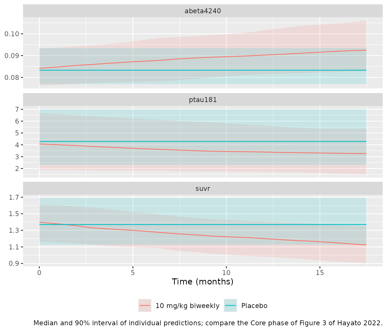
# Placebo profiles stay at their individual baselines (the untreated turnover
# is at steady state; the p-tau181 0.01 ug/mL offset moves it by 0.003%).
plac <- vpc |>
  dplyr::filter(scenario == "Placebo") |>
  dplyr::group_by(endpoint, id) |>
  dplyr::summarise(drift = max(abs(value / value[time == 0] - 1)), .groups = "drop")
stopifnot(all(plac$drift < 1e-3))
Assumptions and deviations
-
APOE4 coding of the SUVr baseline effect. The Table
2 footnote reads “APOE = 0 (APOE4 carrier) or 1 (non-carrier)”, which
would make non-carriers 4% higher. The Table 2 row label (“APOE4 carrier
~ baseline”), the Results (“APOE4 carrier subjects have higher baseline
SUVr”) and the Discussion (“APOE4 carriers have slightly higher baseline
SUVr than non-carriers”) all make carriers the 1-level, so the
maintainers treat the footnote as an inversion and apply the 1.04 ratio
to
APOE4_CARRIER = 1. - Baseline SUVr / Emax correlation. Table 2 gives R = 0.669 (bootstrap median 0.674); the Results text quotes 0.608. The table value is used.
- p-tau181 baseline equation. The footnote under Table 3 prints the typical baseline as “0.00313 x (BW/72.2)^-0.300”, repeating the slope estimate; Table 3 and Model S4 give the baseline theta as 4.06 pg/mL, which is used.
- Weight normalisation of the PK model. The control stream and the Table 1 equations normalise weight to 73.7 kg; the Figure 2 caption names a 73.4 kg reference subject. 73.7 kg is used.
-
p-tau181 concentration offset. Model S4
$DESdrives the inhibition withC1A + 0.01(ug/mL); Figure 1 prints the equation without the offset. The control-stream form is used; it shifts the untreated steady state by 0.003%. -
Diagnosis and ADA on the p-tau181 baseline. Model
S4 carries both as
THETA = 1 FIXafter backward elimination (Table S10); they have no effect and are not encoded. -
PK residual error. Model S1
$ERRORisW = F + 0.01; Y = W + W*ERR, so the residual SD is sigma x (prediction + 0.01 ug/mL). This is encoded as acombined1()error with the additive SD equal to 0.01 ug/mL times the study-specific proportional SD. The study is selected withSTUDY_LEC101andSTUDY_LEC104(both 0 = study 201). -
Sequential fitting. The paper fitted each PK/PD
model on the post hoc individual PK parameters of the PK model. The
library PK/PD models instead embed the population PK model with its
parameters and IIV fixed, so a simulation draws PK and PD variability
together. Residual error on serum concentration is carried only by
Hayato_2022_lecanemab. - Year length. All three PK/PD control streams convert per-year rate constants with 8760 h per year (365 days); the models do the same.
- Amyloid-negativity simulation. The paper does not state the cohort behind its 64.6% / 36.7% figures beyond “interindividual variabilities of PD parameters”. The maintainers reproduced them with the Figure 4 setting (baseline 1.38, typical PK) and the Emax IIV; with the baseline IIV and the model’s APOE4-dependent baseline switched on as well, the same cohort gives roughly 70% and 47%.
- Virtual cohorts. Covariates are drawn from truncated normal distributions matching the means and SDs of Table S2; sex, APOE4 status and Japanese race are Bernoulli with the Table S2 proportions. ADA status is set negative and Process A material is assumed (Core phase).
- Digitised values. The Figure 2, 4 and 5 comparison values were read off the published figures by the maintainers.
- No correction notice for this article was found on Europe PMC (checked 2026-10-10).