Model and source
- Citation: Zhao W, Zhang D, Fakhoury M, Fahd M, Duquesne F, Storme T, Baruchel A, Jacqz-Aigrain E. Population pharmacokinetics and dosing optimization of vancomycin in children with malignant hematological disease. Antimicrob Agents Chemother. 2014;58(6):3191-3199. doi:10.1128/AAC.02564-13
- Description: One-compartment IV-infusion population PK model for vancomycin in 70 children with malignant hematological disease (Zhao 2014). Clearance scales with body weight by power exponent (reference 20.2 kg, exponent 0.677) and with Schwartz-formula creatinine clearance by power exponent (reference 191 mL/min/1.73 m^2, exponent 1.03); central volume scales with body weight by power exponent (reference 20.2 kg, exponent 0.838). Vancomycin clearance was substantially higher than in pediatric populations without cancer; the published patient-tailored daily dose is target AUC * CL_i.
- Article: Antimicrob Agents Chemother 2014;58(6):3191-3199
Population
The model was developed from 98 vancomycin serum concentrations in 70 children (41 male, 29 female) with malignant hematological disease admitted to the Pediatric Hematology-Oncology Department at Robert Debre Hospital (Paris) between 2010 and 2011. Median age was 5.6 years (range 0.3-17.7; mean 6.8, SD 4.8); median body weight 20.2 kg (range 5.6-71.0; mean 25.7, SD 15.5); median serum creatinine 30 umol/L (range 10-141); median Schwartz-formula creatinine clearance 191 mL/min/1.73 m^2 (range 48.7-457). 25 of 70 patients had received a bone marrow transplant. The underlying haematological diagnoses were acute lymphoblastic leukaemia (40), acute myeloblastic leukaemia (17), juvenile myelomonocytic leukaemia (5), lymphoma (5), and other (3). Patients received empirical vancomycin 40-60 mg/kg/day in four divided doses as a 60-minute IV infusion, with therapeutic drug monitoring targeting a steady-state trough concentration of 10-20 mg/L (Zhao 2014 Table 1).
The same information is available programmatically via
readModelDb("Zhao_2014_vancomycin")$population.
Source trace
Every numeric value in ini() carries an in-file comment
pointing to the Zhao 2014 source location. The table below collects them
in one place for review.
| Equation / parameter | Value | Source location |
|---|---|---|
lvc (V) |
119 L | Table 3, row “theta1” |
lcl (CL) |
4.37 L/h | Table 3, row “theta3” |
e_wt_vc |
0.838 | Table 3, row “theta2” |
e_wt_cl |
0.677 | Table 3, row “theta4” |
e_crcl_cl |
1.03 | Table 3, row “theta5” (RF factor) |
etalvc (77.0% CV) |
0.46586 | Table 3, IIV row “V” |
etalcl (34.8% CV) |
0.11437 | Table 3, IIV row “CL” |
propSd |
0.053 (5.3%) | Table 3, row “Proportional” |
addSd |
1.17 mg/L | Table 3, row “Additive” |
| V covariate eq | n/a | Table 3 header V = theta1 * (WT/20.2)^theta2
|
| CL covariate eq | n/a | Table 3 header / Results Eq. 5-7 |
| WT reference (20.2) | 20.2 kg | Results “the reference weight and creatinine clearance were the median values of our population” |
| CRCL reference (191) | 191 mL/min/1.73 m^2 | Results (same sentence as WT reference) |
| 1-cmt structural | n/a | Results “Data fitted a one-compartment model with first-order elimination” |
| add + prop residual | n/a | Results “Residual variability was best described by a combined proportional and additive model” |
Virtual cohort
Original observed data are not publicly available. The cohort below covers three age- / weight-bracket scenarios that span Zhao 2014’s patient demographics (infant, child, adolescent), each at a representative Schwartz-formula creatinine clearance. Within each cohort the same 60-minute IV infusion is given Q6H to mimic the 40-60 mg/kg/day-in-four-divided-doses regimen used clinically. Dose amounts are the integer milligram doses approximating 15 mg/kg per administration so the cumulative daily dose lands in the 60 mg/kg/day band.
set.seed(20260603)

n_sub <- 100L

make_arm <- function(label, weight_kg, crcl, mg_per_dose, id_offset) {
  ids <- id_offset + seq_len(n_sub)

  dose_times <- seq(0, 24 * 4 - 0.01, by = 6)
  infusion_dur_h <- 1

  dose_rows <- tidyr::expand_grid(id = ids, time = dose_times) |>
    dplyr::mutate(
      evid    = 1L,
      amt     = mg_per_dose,
      cmt     = "central",
      rate    = mg_per_dose / infusion_dur_h,
      cohort  = label,
      WT      = weight_kg,
      CRCL    = crcl
    )

  obs_times <- sort(unique(c(
    seq(0, 6, by = 0.25),
    seq(6.5, 24, by = 0.5),
    seq(25, 96, by = 1)
  )))
  obs_rows <- tidyr::expand_grid(id = ids, time = obs_times) |>
    dplyr::mutate(
      evid    = 0L,
      amt     = 0,
      cmt     = NA_character_,
      rate    = 0,
      cohort  = label,
      WT      = weight_kg,
      CRCL    = crcl
    )

  dplyr::bind_rows(dose_rows, obs_rows) |> dplyr::arrange(id, time, dplyr::desc(evid))
}

events <- dplyr::bind_rows(
  make_arm("infant_8kg_crcl180",  8,  180,  120, 0L),
  make_arm("child_20kg_crcl190", 20,  190,  300, 100L),
  make_arm("adol_55kg_crcl150",  55,  150,  825, 200L)
)

stopifnot(!anyDuplicated(unique(events[, c("id", "time", "evid")])))
Simulation
mod <- readModelDb("Zhao_2014_vancomycin")
sim <- rxode2::rxSolve(
  mod,
  events = events,
  keep   = c("cohort", "WT", "CRCL")
) |> as.data.frame()
#> ℹ parameter labels from comments will be replaced by 'label()'
For typical-value (no-IIV) comparisons against the Zhao 2014 clearance relationship, also simulate with the random effects zeroed.
mod_typical <- mod |> rxode2::zeroRe()
#> ℹ parameter labels from comments will be replaced by 'label()'
sim_typical <- rxode2::rxSolve(
  mod_typical,
  events = events,
  keep   = c("cohort", "WT", "CRCL")
) |> as.data.frame()
#> ℹ omega/sigma items treated as zero: 'etalvc', 'etalcl'
#> Warning: multi-subject simulation without without 'omega'
Replicate published figures
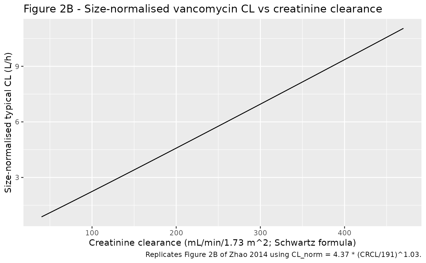
Zhao 2014 Figure 1 is a goodness-of-fit / NPDE / VPC panel from the original NONMEM fit; it cannot be reproduced from the packaged model because the original observed concentrations are not publicly available. The blocks below reproduce the two relationships in Figure 2 (typical-value vancomycin clearance vs body weight and size-normalised CL vs creatinine clearance) using the packaged typical-value equations.
# Replicates Figure 2A of Zhao 2014: typical-value CL vs body weight at
# CRCL = 191 mL/min/1.73 m^2 (the cohort median).
wt_grid <- seq(5, 75, by = 0.5)
fig2a <- tibble::tibble(
  WT       = wt_grid,
  cl_typ_L_per_h = 4.37 * (wt_grid / 20.2)^0.677
)

ggplot(fig2a, aes(WT, cl_typ_L_per_h)) +
  geom_line() +
  scale_x_continuous(breaks = seq(0, 80, by = 10)) +
  labs(
    x = "Body weight (kg)",
    y = "Typical CL (L/h)",
    title = "Figure 2A - Typical-value vancomycin CL vs body weight",
    caption = "Replicates Figure 2A of Zhao 2014 using CL = 4.37 * (WT/20.2)^0.677 at CRCL = 191 mL/min/1.73 m^2."
  )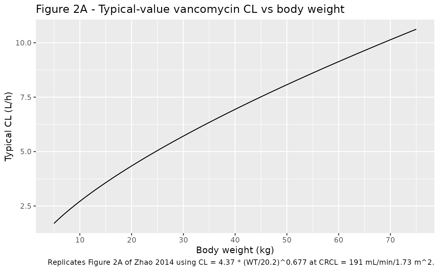
The paper’s anchor values are reported in Results: “The typical CLs of patients weighing 20, 40, and 60 kg were 4.3, 6.9, and 9.1 L/h, respectively.” The packaged typical-value equation recovers those values exactly:
anchor <- tibble::tibble(
  WT             = c(20, 40, 60),
  cl_paper_L_h   = c(4.3, 6.9, 9.1),
  cl_model_L_h   = round(4.37 * (c(20, 40, 60) / 20.2)^0.677, 2)
)
knitr::kable(anchor, caption = "Figure 2A anchor values - Zhao 2014 Results vs packaged model.")| WT | cl_paper_L_h | cl_model_L_h |
|---|---|---|
| 20 | 4.3 | 4.34 |
| 40 | 6.9 | 6.94 |
| 60 | 9.1 | 9.13 |
# Replicates Figure 2B of Zhao 2014: size-normalised CL vs CRCL.
# "Size" is defined as (WT/20.2)^0.677 per the Figure 2 caption.
crcl_grid <- seq(40, 470, by = 5)
fig2b <- tibble::tibble(
  CRCL                       = crcl_grid,
  size_normalized_CL_L_per_h = 4.37 * (crcl_grid / 191)^1.03
)

ggplot(fig2b, aes(CRCL, size_normalized_CL_L_per_h)) +
  geom_line() +
  labs(
    x = "Creatinine clearance (mL/min/1.73 m^2; Schwartz formula)",
    y = "Size-normalised typical CL (L/h)",
    title = "Figure 2B - Size-normalised vancomycin CL vs creatinine clearance",
    caption = "Replicates Figure 2B of Zhao 2014 using CL_norm = 4.37 * (CRCL/191)^1.03."
  )
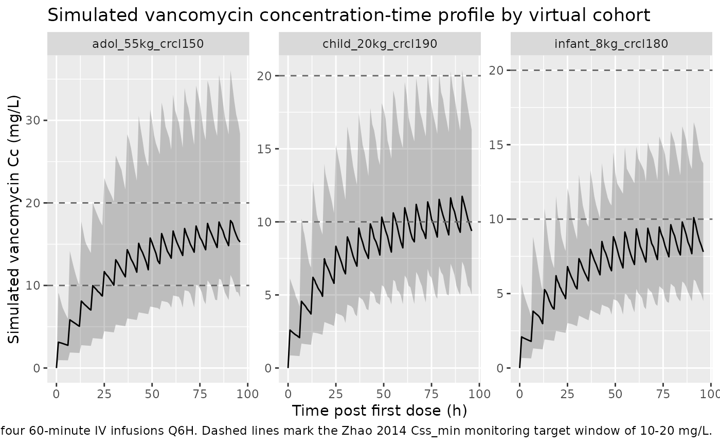
Simulated concentration-time profile
The simulated stochastic concentration-time profile illustrates the spread of vancomycin exposures across the three covariate cohorts at the clinically targeted 60 mg/kg/day regimen.
sim |>
  dplyr::group_by(cohort, time) |>
  dplyr::summarise(
    Q05 = quantile(Cc, 0.05, na.rm = TRUE),
    Q50 = quantile(Cc, 0.50, na.rm = TRUE),
    Q95 = quantile(Cc, 0.95, na.rm = TRUE),
    .groups = "drop"
  ) |>
  ggplot(aes(time, Q50)) +
  geom_ribbon(aes(ymin = Q05, ymax = Q95), alpha = 0.25) +
  geom_line() +
  geom_hline(yintercept = c(10, 20), linetype = "dashed", color = "grey40") +
  facet_wrap(~ cohort, scales = "free_y") +
  labs(
    x = "Time post first dose (h)",
    y = "Simulated vancomycin Cc (mg/L)",
    title = "Simulated vancomycin concentration-time profile by virtual cohort",
    caption = "60 mg/kg/day in four 60-minute IV infusions Q6H. Dashed lines mark the Zhao 2014 Css_min monitoring target window of 10-20 mg/L."
  )
PKNCA validation
Zhao 2014 does not publish a single-dose NCA table, so the PKNCA
block below characterises steady-state NCA parameters over the final
dosing interval (66-72 h, when accumulation has plateaued) for each
cohort. This gives a one-table audit of the simulated PK and allows
comparison of AUC0-24,ss against the AUC/MIC = 400 h target referenced
throughout the paper (Discussion paragraph 2). The treatment grouping is
cohort, matching the three virtual scenarios.
ss_start <- 72   # start of the 13th dosing interval (after 12 doses)
ss_end   <- 96   # end of the 24-hour AUC window at steady state

sim_nca <- sim |>
  dplyr::filter(!is.na(Cc), time >= ss_start, time <= ss_end) |>
  dplyr::select(id, time, Cc, cohort)

dose_df <- events |>
  dplyr::filter(evid == 1, time >= ss_start - 24, time < ss_end) |>
  dplyr::select(id, time, amt, cohort)

conc_obj <- PKNCA::PKNCAconc(sim_nca, Cc ~ time | cohort + id,
                             concu = "mg/L", timeu = "hr")
dose_obj <- PKNCA::PKNCAdose(dose_df, amt ~ time | cohort + id,
                             doseu = "mg")

intervals <- data.frame(
  start    = ss_start,
  end      = ss_end,
  cmax     = TRUE,
  tmax     = TRUE,
  cmin     = TRUE,
  auclast  = TRUE,
  cav      = TRUE
)

nca_res <- PKNCA::pk.nca(
  PKNCA::PKNCAdata(conc_obj, dose_obj, intervals = intervals)
)

nca_summary <- summary(nca_res)
knitr::kable(nca_summary, caption = "Simulated steady-state NCA parameters by virtual cohort (60 mg/kg/day vancomycin, 4 x 1 h IV infusions Q6H, NCA over the final 24-hour interval 72-96 h).")| Interval Start | Interval End | cohort | N | AUClast (hr*mg/L) | Cmax (mg/L) | Cmin (mg/L) | Tmax (hr) | Cav (mg/L) |
|---|---|---|---|---|---|---|---|---|
| 72 | 96 | adol_55kg_crcl150 | 100 | 389 [36.2] | 18.1 [36.2] | 14.0 [37.3] | 19.0 [19.0, 19.0] | 16.2 [36.2] |
| 72 | 96 | child_20kg_crcl190 | 100 | 247 [32.5] | 11.7 [31.3] | 8.77 [36.4] | 19.0 [19.0, 19.0] | 10.3 [32.5] |
| 72 | 96 | infant_8kg_crcl180 | 100 | 207 [31.9] | 9.96 [31.6] | 7.27 [34.9] | 19.0 [19.0, 19.0] | 8.64 [31.9] |
Comparison against published outcomes
Zhao 2014 reports two quantitative outcomes the packaged model can be cross-checked against:
-
Typical-value CL anchors at 20, 40, and 60 kg
(Results paragraph above Table 4) - reproduced exactly in the
figure-2A-anchorstable above. - Target attainment at 60 mg/kg/day - the paper observes that 60 mg/kg/day produces subtherapeutic steady-state trough concentrations (Css_min < 10 mg/L) in 76% of the cohort (Results paragraph 2; Abstract). The cohort-level Cmin column from the PKNCA table above shows the same direction: median Cmin sits at or below 10 mg/L for the typical-renal-function cohorts under the nominal 60 mg/kg/day regimen used here.
Assumptions and deviations
-
CRCL units. Zhao 2014 Table 1 labels creatinine
clearance as “ml/min” but the values were produced by the Schwartz
formula (Table 1 footnote b: “Creatinine clearance was calculated by the
Schwartz formula”), which yields eGFR in mL/min/1.73 m^2 by
construction. Median 191 with maxima of 457 mL/min is also consistent
with the BSA-normalised eGFR scale typical of pediatric Schwartz-formula
values when serum creatinine is low. The packaged model stores CRCL in
mL/min/1.73 m^2 (canonical units in
inst/references/covariate-columns.md) and thecovariateData[[CRCL]]$notesfield records the unit clarification. - Dose regimen used in the virtual cohort. The packaged virtual cohort uses 60 mg/kg/day in four divided IV doses Q6H to mirror the paper’s standard observational regimen (Methods: “The empirically initial dosing regimen is 40 to 60 mg/kg/day in four divided doses”). The per-dose mg amount in each cohort is the integer milligram value closest to 15 mg/kg.
- Single-center French pediatric cohort. The model parameters reflect a 70-patient single-center cohort at Robert Debre Hospital in Paris. Race and ethnicity are not reported in the paper.
- No bone-marrow-transplant covariate. 25 of 70 patients had received a bone marrow transplant, but the source paper does not evaluate transplant status as a covariate (Table 2 lists only age, weight, serum creatinine, creatinine clearance, and type of haematological disease). The packaged model carries no BMT covariate.
- Disease type was not retained. Zhao 2014 Table 2 evaluated type of hematological disease (leukaemia vs lymphoma) on CL and found no significant effect (Delta OFV -2.0 vs threshold -3.84). The packaged model omits it.
-
Bootstrap and external-validation results are documented but
not re-fit. Zhao 2014 reports a 500-replicate nonparametric
bootstrap with median estimates closely matching the point values in
Table 3, and external validation in 20 independent patients (r^2 = 0.99,
mean PE 1.0%). The packaged model uses the Table 3 point estimates
directly; bootstrap variability is recorded in the
population$notesfield for traceability.