Vancomycin in class 3 obesity, parametric vs nonparametric (Hughes 2024)
Source:vignettes/articles/Hughes_2024_vancomycin.Rmd
Hughes_2024_vancomycin.RmdModel and source
Hughes 2024 is a quality-improvement effort that fitted two population PK models to the same vancomycin therapeutic-drug-monitoring dataset from a single institution, in order to ask whether a parametric or a nonparametric estimation method produces the better model for model-informed precision dosing (MIPD). Both models are packaged here.
mod_par <- readModelDb("Hughes_2024_vancomycin_parametric")
mod_np <- readModelDb("Hughes_2024_vancomycin_nonparametric")- Parametric (nlmixr2 SAEM): Two-compartment intravenous population PK model for vancomycin in hospitalized adults with class 3 obesity (BMI >= 40 kg/m2), developed as a parametric (maximum-likelihood) fit with nlmixr2 SAEM. Fat-free mass is computed inside the model by the Janmahasatian equations from body weight, height and sex; creatinine clearance is then computed by a Cockcroft-Gault form that substitutes fat-free mass for total body weight. Clearance scales as (CRCL/100)^0.887 with no allometric term of its own; central and peripheral volumes scale linearly on (FFM/70). Intercompartmental clearance carries neither a covariate nor an eta. This is the parametric half of a parametric-versus-nonparametric comparison fitted to a single institution’s routine therapeutic-drug-monitoring data; the nonparametric counterpart is modellib(‘Hughes_2024_vancomycin_nonparametric’).
- Nonparametric (Pmetrics NPAG): Two-compartment intravenous population PK model for vancomycin in hospitalized adults with class 3 obesity (BMI >= 40 kg/m2), developed as a NONPARAMETRIC fit with Pmetrics using the nonparametric adaptive grid (NPAG) algorithm. Structurally identical to its parametric sibling: fat-free mass is computed inside the model by the Janmahasatian equations from body weight, height and sex, creatinine clearance is then computed by a Cockcroft-Gault form that substitutes fat-free mass for total body weight, clearance scales as (CRCL/100)^1.05, and both volumes scale linearly on (FFM/70). Unlike the parametric fit, between-subject variability is carried on all four disposition parameters including intercompartmental clearance, and the residual error is a fixed Pmetrics assay-error polynomial rather than an estimated proportional term. NPAG estimates a discrete joint distribution of individual parameters that has no closed form; it is approximated here by independent lognormal marginals, so the shape of the joint density is not recoverable from this encoding. The parametric counterpart is modellib(‘Hughes_2024_vancomycin_parametric’).
- Citation: Hughes MSA, Hughes JH, Endicott J, Langton M, Ahern JW, Keizer RJ. Developing parametric and nonparametric models for model-informed precision dosing: a quality improvement effort in vancomycin for patients with obesity. Ther Drug Monit 2024;46(5):575-583. doi:10.1097/FTD.0000000000001214. Parameter estimates from Table 2, nlmixr2 (SAEM) column; structural model from the Table 2 footnote and from Supplemental Digital Content 1 sections S3 (nlmixr2 model code) and S4 (NONMEM control stream), http://links.lww.com/TDM/A753. The fat-free-mass equations are Janmahasatian S, Duffull SB, Ash S, Ward LC, Byrne NM, Green B. Quantification of lean bodyweight. Clin Pharmacokinet 2005;44(10):1051-1065.
- Article: https://doi.org/10.1097/FTD.0000000000001214
- Supplement (Supplemental Digital Content 1): http://links.lww.com/TDM/A753
The paper also fitted the parametric model a third time in NONMEM as
a software cross-check, and reports that parameter set in Table 2 as
well. It is not packaged again here: the Results state “we present only
the results for nlmixr2”, Table 3 (“Comparison of Final Models”)
enumerates exactly two final models, and the NONMEM parameter set is
already available in this library as
modellib("Tong_2026_vancomycin_hughes"), transcribed from
the control stream in the Tong 2026 supplement. See the Errata below,
where the three parametric parameter sets are compared side by side.
Population
Both models were fitted to the same 83 patients contributing 272 vancomycin TDM levels (median 2 per patient, range 1-29; 31 peaks, 115 troughs, 126 random), collected at the University of Vermont Medical Center between 1 November 2021 and 14 February 2023 and exported from the InsightRX Nova precision-dosing software. Inclusion required a body mass index of at least 40 kg/m^2 at some point during treatment and at least one vancomycin level. Median age was 56.3 years (range 24.2-89.3), median weight 134 kg (range 91.6-218), median BMI 46.3 kg/m^2 (range 40-70.3), median serum creatinine 0.84 mg/dL (range 0.40-2.51), and the cohort was 42/83 female. Race and ethnicity were not reported, and the Discussion records as a limitation that patient status, level of care and indication for vancomycin were not collected. Three levels were removed during data cleaning; all remaining levels were above the lower limit of quantification. (Table 1, development-dataset column.)
A separate external validation dataset of 576 patients across 74 US organizations (1191 levels) was used to compare the parametric model’s predictive performance against four published obesity models, but was not used to estimate any parameter.
The same information is available programmatically via each model’s
population metadata
(rxode2::rxode(readModelDb("Hughes_2024_vancomycin_parametric"))$population).
Source trace
The per-parameter origin is recorded as an in-file comment next to
each ini() entry in
inst/modeldb/specificDrugs/Hughes_2024_vancomycin_parametric.R
and ..._nonparametric.R. The table below collects them in
one place. “Table 2 (par.)” and “Table 2 (np.)” refer to the nlmixr2
(SAEM) and Pmetrics columns of Table 2 respectively; “SDC1 Sn of Supplemental Digital Content 1.
| Equation / parameter | Parametric | Nonparametric | Source location |
|---|---|---|---|
lcl (CL at CrCl 100 mL/min) |
log(5.09) L/h |
log(6.74) L/h |
Table 2, CL row |
lvc (Vc at FFM 70 kg) |
log(64.9) L |
log(104) L |
Table 2, Vc row |
lq (Q) |
log(6.36) L/h |
log(7.5) L/h |
Table 2, Q row |
lvp (Vp at FFM 70 kg) |
log(66.4) L |
log(142) L |
Table 2, Vp row |
e_crcl_cl (exponent on CrCl/100) |
0.887 |
1.05 |
Table 2, u3 row |
e_ffm_vc_vp (exponent on FFM/70) |
fixed(1) |
fixed(1) |
Table 2, u2 row (FIX) |
etalcl |
0.249^2 |
log(0.222^2+1) |
Table 2, CL BSV (24.9 / 22.2 %CV) |
etalvc |
0.178^2 |
log(0.252^2+1) |
Table 2, Vc BSV (17.8 / 25.2 %CV) |
etalq |
absent | log(0.54^2+1) |
Table 2, Q BSV (“-” / 54 %CV); Table 3 |
etalvp |
0.803^2 |
log(0.350^2+1) |
Table 2, Vp BSV (80.3 / 35.0 %CV) |
propSd |
0.168 |
fixed(0.1) |
Table 2, RUV row |
addSd |
fixed(0.001) |
fixed(0.5) |
SDC1 S3 / S4 (par.); Table 2 RUVadd (np.) |
| Error combination | quadrature | combined1() |
SDC1 S4 W = SQRT(...); S5 #Err
polynomial |
Covariate model CLi, Vi, Qi,
Vp,i
|
n/a | n/a | Table 2 footnote; SDC1 S4 $PK; S5
#Sec
|
| BMI, FFM (Janmahasatian), Cockcroft-Gault on FFM | n/a | n/a | Methods/Data Collection; SDC1 S4 $PK
|
| Structural model: 2-compartment IV | n/a | n/a | Methods/Model Development; Table 3 |
The allometric exponent u1 that appears in the Table 2
footnote (CLi = CL*(FFM/70)^u1*(CrCL/100)^u3,
Qi = Q*(FFM/70)^u1) is not part of either
final model: it has no row in Table 2, the Results state for the
parametric fit that it “considerably worsened the model fit when fixed
and was estimated to be close to zero when estimated; therefore, this
exponent was excluded” and for the nonparametric fit that “once CrCl was
included as a predictor of CL, the inclusion of the allometric exponent
on CL and Q did not improve the model and was, therefore, removed”,
Table 3 lists the final covariates as CL~CrCl / Vc~FFM / Vp~FFM only,
and the SDC1 S4 $PK and S5 #Sec blocks both
write Q with no covariate term. Both packaged models therefore set
u1 = 0.
Structural comparison (reproduces Table 3)
Table 3’s “Model structure” rows are recovered directly from the two packaged model objects, which is a check that the encoding carries the paper’s one structural difference between the approaches: the nonparametric fit puts between-subject variability on all four disposition parameters, the parametric fit on only three.
struct_row <- function(mod, label) {
  ui <- rxode2::rxode(mod)
  etas <- ui$iniDf$name[!is.na(ui$iniDf$neta1)]
  tibble(
    Approach   = label,
    Structural = "2-compartment",
    Covariates = "CL ~ CrCl; Vc ~ FFM; Vp ~ FFM",
    BSV        = paste(sub("^etal", "", etas), collapse = ", "),
    `Residual error` = ui$predDf$addProp
  )
}

structure_tbl <- bind_rows(
  struct_row(mod_par, "Parametric (nlmixr2)"),
  struct_row(mod_np,  "Nonparametric (Pmetrics)")
)

knitr::kable(structure_tbl, caption = "Reproduces the 'Model structure' rows of Table 3 of Hughes 2024.")| Approach | Structural | Covariates | BSV | Residual error |
|---|---|---|---|---|
| Parametric (nlmixr2) | 2-compartment | CL ~ CrCl; Vc ~ FFM; Vp ~ FFM | cl, vc, vp | default |
| Nonparametric (Pmetrics) | 2-compartment | CL ~ CrCl; Vc ~ FFM; Vp ~ FFM | cl, vc, q, vp | combined1 |
# Table 3 states BSV on "CL, Vc, Vp" (parametric) and "CL, Vc, Q, Vp" (nonparametric).
stopifnot(
  structure_tbl$BSV[structure_tbl$Approach == "Parametric (nlmixr2)"] == "cl, vc, vp",
  structure_tbl$BSV[structure_tbl$Approach == "Nonparametric (Pmetrics)"] == "cl, vc, q, vp"
)
Virtual cohort
Original observed data are not publicly available. The cohort below
is drawn to match the Table 1 development-dataset demographics. Height
and BMI are sampled and weight is derived as
WT = BMI * (HT/100)^2, which is the same relation the model
uses internally; this reproduces the published median weight without
having to sample weight and height as if they were independent.
# set.seed() seeds R's RNG (used for the covariate draws below). It does NOT seed
# rxode2's simulation RNG, whose streams are partitioned per solver thread -- so the
# IIV draws in the VPC section differ between a 2-core CI runner and a 16-thread
# workstation. Every assertion below is written to hold for any cohort the model can
# produce.
set.seed(20240905)
n_subj <- 200L  # per model arm; cohorts are capped at 200/arm

clamp <- function(x, lo, hi) pmin(pmax(x, lo), hi)

cohort <- tibble(
  id    = seq_len(n_subj),
  HT    = clamp(rnorm(n_subj, 170, 11),           122,   190),   # Table 1: 170 (122-190) cm
  BMI   = clamp(40 + rlnorm(n_subj, log(6.3), .65), 40,   70.3), # Table 1: 46.3 (40-70.3)
  AGE   = clamp(rnorm(n_subj, 56.3, 15),          24.2,  89.3),  # Table 1: 56.3 (24.2-89.3)
  SEXF  = rbinom(n_subj, 1, 42 / 83),                            # Table 1: 42/83 female
  CREAT = clamp(rlnorm(n_subj, log(0.84), 0.35),  0.40,  2.51)   # Table 1: 0.84 (0.40-2.51)
) |>
  mutate(WT = BMI * (HT / 100)^2)
Covariate machinery check (reproduces Table 1)
The Janmahasatian fat-free-mass equations and the
Cockcroft-Gault-on-FFM creatinine clearance are computed inside
the model, so they are not visible in ini() and are not
covered by the parameter source-trace. Table 1 nevertheless reports the
resulting cohort medians for both creatinine-clearance
flavours – 84.1 mL/min on fat-free mass and 174 mL/min on total body
weight – which is enough to test the derivation independently.
Recomputing them here with the same equations the model body uses is a
direct check on that machinery.
ffm_of  <- function(WT, BMI, SEXF) {
  ifelse(SEXF == 1, 9270 * WT / (8780 + 244 * BMI), 9270 * WT / (6680 + 216 * BMI))
}
crcl_of <- function(size, AGE, SEXF, CREAT) (140 - AGE) * size * 0.85^SEXF / (72 * CREAT)

cohort <- cohort |>
  mutate(
    FFM      = ffm_of(WT, BMI, SEXF),
    CRCL_FFM = crcl_of(FFM, AGE, SEXF, CREAT),
    CRCL_TBW = crcl_of(WT,  AGE, SEXF, CREAT)
  )

table1 <- tibble::tribble(
  ~Characteristic,                       ~Published, ~Simulated,
  "Weight (kg)",                              134,   median(cohort$WT),
  "Height (cm)",                              170,   median(cohort$HT),
  "BMI (kg/m^2)",                            46.3,   median(cohort$BMI),
  "Age (years)",                             56.3,   median(cohort$AGE),
  "Serum creatinine (mg/dL)",                0.84,   median(cohort$CREAT),
  "Creatinine clearance on TBW (mL/min)",     174,   median(cohort$CRCL_TBW),
  "Creatinine clearance on FFM (mL/min)",    84.1,   median(cohort$CRCL_FFM)
) |>
  mutate(`% diff` = 100 * (Simulated - Published) / Published)

knitr::kable(table1, digits = 1,
caption = "Virtual-cohort medians against the Table 1 development-dataset medians of Hughes 2024.")| Characteristic | Published | Simulated | % diff |
|---|---|---|---|
| Weight (kg) | 134.0 | 134.8 | 0.6 |
| Height (cm) | 170.0 | 170.7 | 0.4 |
| BMI (kg/m^2) | 46.3 | 46.1 | -0.5 |
| Age (years) | 56.3 | 57.2 | 1.6 |
| Serum creatinine (mg/dL) | 0.8 | 0.8 | -4.1 |
| Creatinine clearance on TBW (mL/min) | 174.0 | 170.2 | -2.2 |
| Creatinine clearance on FFM (mL/min) | 84.1 | 85.1 | 1.2 |
# The two creatinine-clearance rows are the load-bearing ones: they exercise the
# Janmahasatian FFM equations and the Cockcroft-Gault substitution. A mis-transcribed
# FFM coefficient or a Cockcroft-Gault written on total body weight moves them by a
# factor of ~2 (the published TBW/FFM ratio is 174/84.1 = 2.07), so a 15% band still
# goes red on any such error while absorbing the sampling noise of a 200-subject draw.
stopifnot(all(abs(table1$`% diff`) < 15))
Typical-value parameters (reproduces Table 2 and the Figure 2 claim)
Evaluating each model at a fixed covariate profile recovers the Table 2 estimates when that profile sits at the models’ reference points (FFM = 70 kg, CrCl = 100 mL/min), and lets the two approaches be compared at the cohort’s median profile. The paper’s Figure 2 / Discussion claim is that “on an average, Pmetrics estimated higher values of CL and V than nlmixr2”.
tv_of <- function(mod, crcl, ffm) {
  th <- rxode2::rxode(mod)$theta
  c(CL = unname(exp(th[["lcl"]]) * (crcl / 100)^th[["e_crcl_cl"]]),
    Vc = unname(exp(th[["lvc"]]) * (ffm / 70)^th[["e_ffm_vc_vp"]]),
    Q  = unname(exp(th[["lq"]])),
    Vp = unname(exp(th[["lvp"]]) * (ffm / 70)^th[["e_ffm_vc_vp"]]))
}

# At the reference profile the covariate terms are 1, so this must return Table 2.
ref_tbl <- bind_rows(
  c(Approach = "Parametric (nlmixr2)",     tv_of(mod_par, crcl = 100, ffm = 70)),
  c(Approach = "Nonparametric (Pmetrics)", tv_of(mod_np,  crcl = 100, ffm = 70))
) |>
  mutate(across(-Approach, as.numeric))

knitr::kable(ref_tbl, digits = 2,
caption = "Model parameters at the reference profile (FFM = 70 kg, CrCl = 100 mL/min); these are the Table 2 estimates of Hughes 2024.")| Approach | CL | Vc | Q | Vp |
|---|---|---|---|---|
| Parametric (nlmixr2) | 5.09 | 64.9 | 6.36 | 66.4 |
| Nonparametric (Pmetrics) | 6.74 | 104.0 | 7.50 | 142.0 |
# Deterministic: a pure function of the ini() values, so an exact check is correct here.
stopifnot(
  isTRUE(all.equal(as.numeric(ref_tbl[1, c("CL", "Vc", "Q", "Vp")]), c(5.09, 64.9, 6.36, 66.4))),
  isTRUE(all.equal(as.numeric(ref_tbl[2, c("CL", "Vc", "Q", "Vp")]), c(6.74, 104,  7.50, 142 )))
)
med_ffm  <- median(cohort$FFM)
med_crcl <- median(cohort$CRCL_FFM)

med_tbl <- bind_rows(
  c(Approach = "Parametric (nlmixr2)",     tv_of(mod_par, med_crcl, med_ffm)),
  c(Approach = "Nonparametric (Pmetrics)", tv_of(mod_np,  med_crcl, med_ffm))
) |>
  mutate(across(-Approach, as.numeric))

knitr::kable(med_tbl, digits = 2,
             caption = sprintf(
               "Model parameters at the cohort median profile (FFM = %.1f kg, CrCl = %.1f mL/min).",
med_ffm, med_crcl))| Approach | CL | Vc | Q | Vp |
|---|---|---|---|---|
| Parametric (nlmixr2) | 4.41 | 62.66 | 6.36 | 64.11 |
| Nonparametric (Pmetrics) | 5.69 | 100.41 | 7.50 | 137.10 |
# Figure 2 / Discussion: "On an average, Pmetrics estimated higher values of CL and V
# than nlmixr2." This is a comparison of two DETERMINISTIC functions of the published
# ini() values at a common covariate profile -- not a race between two noisy simulated
# statistics -- so a strict ordering assertion is legitimate here. It holds at every
# covariate profile, because the nonparametric CL and Vc exceed the parametric ones at
# the reference point and the covariate terms are shared.
stopifnot(
  med_tbl$CL[2] > med_tbl$CL[1],
  med_tbl$Vc[2] > med_tbl$Vc[1]
)
Closed-form validation: AUC0-inf equals Dose / CL
Neither model’s source paper reports an NCA table, so there is no
published Cmax / AUC / half-life to compare against. What is
available is the exact identity that a linear two-compartment model must
satisfy: after a single intravenous dose, AUC0-inf equals
Dose / CL, where CL is computed independently
from the published ini() values and the covariate
equations. Simulating with the random effects zeroed makes this a
deterministic check of the whole chain – covariate derivation, parameter
scaling, ODE system, and observation equation – against a quantity that
never touches the solver.
# A single median-profile subject per model, dosed 2000 mg as a 2-hour infusion.
ref_subj <- list(WT = 134, HT = 170, AGE = 56.3, SEXF = 0, CREAT = 0.84)
dose_amt <- 2000

# Observations are written on the ODE state "central" -- NEVER on the observable "Cc",
# which would auto-inject a cmt() slot after the ODE states and renumber them.
ev_single <- rxode2::et(amt = dose_amt, dur = 2, cmt = "central") |>
  rxode2::et(seq(0, 480, by = 0.25), cmt = "central")

solve_typical <- function(mod) {
  rxode2::rxSolve(rxode2::zeroRe(mod), ev_single,
                  params = unlist(ref_subj), returnType = "data.frame")
}

sim_single <- bind_rows(
  solve_typical(mod_par) |> mutate(Approach = "Parametric (nlmixr2)",     id = 1L),
  solve_typical(mod_np)  |> mutate(Approach = "Nonparametric (Pmetrics)", id = 2L)
)
#> ℹ omega/sigma items treated as zero: 'etalcl', 'etalvc', 'etalvp'
#> ℹ omega/sigma items treated as zero: 'etalcl', 'etalvc', 'etalq', 'etalvp'
sim_nca <- sim_single |>
  dplyr::filter(!is.na(Cc)) |>
  dplyr::select(id, time, Cc, Approach)

# Guarantee a time = 0 row per (id, Approach). For an IV infusion the pre-dose
# concentration is 0, and PKNCA needs the row to anchor AUC from the interval start.
sim_nca <- bind_rows(
  sim_nca,
  sim_nca |> distinct(id, Approach) |> mutate(time = 0, Cc = 0)
) |>
  distinct(id, Approach, time, .keep_all = TRUE) |>
  arrange(id, Approach, time)

dose_df <- tibble(id = c(1L, 2L), time = 0,  amt = dose_amt,
                  Approach = c("Parametric (nlmixr2)", "Nonparametric (Pmetrics)"))

conc_obj <- PKNCA::PKNCAconc(as.data.frame(sim_nca), Cc ~ time | Approach + id,
                             concu = "mg/L", timeu = "h")
dose_obj <- PKNCA::PKNCAdose(as.data.frame(dose_df), amt ~ time | Approach + id,
                             doseu = "mg")

intervals <- data.frame(start = 0, end = Inf,
                        cmax = TRUE, tmax = TRUE, aucinf.obs = TRUE, half.life = TRUE)

nca_single <- PKNCA::pk.nca(PKNCA::PKNCAdata(conc_obj, dose_obj, intervals = intervals))
# Reference side: the closed-form values, computed from the published ini() numbers and
# the paper's covariate equations WITHOUT touching the solver output, so the comparison
# can actually go red.
bmi_ref  <- ref_subj$WT / (ref_subj$HT / 100)^2
ffm_ref  <- ffm_of(ref_subj$WT, bmi_ref, ref_subj$SEXF)
crcl_ref <- crcl_of(ffm_ref, ref_subj$AGE, ref_subj$SEXF, ref_subj$CREAT)

closed_form <- lapply(
  list("Parametric (nlmixr2)" = mod_par, "Nonparametric (Pmetrics)" = mod_np),
  function(m) {
    p   <- tv_of(m, crcl_ref, ffm_ref)
    kel <- p[["CL"]] / p[["Vc"]]; k12 <- p[["Q"]] / p[["Vc"]]; k21 <- p[["Q"]] / p[["Vp"]]
    b   <- kel + k12 + k21
    lz  <- (b - sqrt(b^2 - 4 * kel * k21)) / 2   # terminal (beta) rate constant
    c(aucinf.obs = dose_amt / p[["CL"]], half.life = log(2) / lz)
  })

reference <- tibble(
  Approach   = names(closed_form),
  aucinf.obs = vapply(closed_form, `[[`, numeric(1), "aucinf.obs"),
  half.life  = vapply(closed_form, `[[`, numeric(1), "half.life")
)

cmp <- nlmixr2lib::ncaComparisonTable(
  simulated     = nca_single,
  reference     = reference,
  by            = "Approach",
  params        = c("aucinf.obs", "half.life"),
  units         = c(aucinf.obs = "mg*h/L", half.life = "h"),
  tolerance_pct = 5
)

knitr::kable(cmp, caption = paste(
  "Simulated NCA against the closed-form identities AUC0-inf = Dose/CL and",
  "t1/2 = ln(2)/beta. The reference column is NOT a published NCA table --",
  "Hughes 2024 reports none -- but is derived from the published ini() values.",
"* marks a difference above 5%."), align = c("l", "l", "r", "r", "r"))| NCA parameter | Approach | Reference | Simulated | % diff |
|---|---|---|---|---|
| AUC0-∞ (obs) (mg*h/L) | Parametric (nlmixr2) | 383 | 383 | -0.0% |
| AUC0-∞ (obs) (mg*h/L) | Nonparametric (Pmetrics) | 288 | 288 | -0.0% |
| t½ (h) | Parametric (nlmixr2) | 23.2 | 23.1 | -0.3% |
| t½ (h) | Nonparametric (Pmetrics) | 35.7 | 35.6 | -0.3% |
# ncaComparisonTable() returns `% diff` as TEXT carrying a "%" suffix and a trailing
# "*" on out-of-tolerance rows, so both must be stripped before a numeric comparison --
# as.numeric("-0.3%") is NA, and all(NA) is NA, which would make this gate un-red-able.
pct <- as.numeric(sub("%$", "", sub("\\*$", "", cmp$`% diff`)))
stopifnot(nrow(cmp) == 4L, !anyNA(pct))   # the gate must have rows to test

# Deterministic quantities: no IIV, no residual error, one fixed covariate profile.
# The only error sources are trapezoidal integration on a 0.25 h grid and PKNCA's
# lambda-z tail extrapolation -- realised 0.0% on AUC and 0.3% on half-life -- so a 2%
# bound is tight enough to catch a mis-scaled volume, a dropped covariate term or a
# wrong error-model combination, all of which move AUC by tens of percent.
stopifnot(all(abs(pct) < 2))
Simulated dosing under the study protocol
The institutional protocol (Methods, Data Collection) gave patients with BMI >= 40 kg/m^2 a 20 mg/kg loading dose capped at 4000 mg, followed by an intermittent-infusion maintenance regimen chosen to reach an AUC of 400-600 mg*h/L. The cohort below is dosed that way – loading dose, then 1000 mg every 12 h for 7 days – and simulated through each model with between-subject variability, giving the visual-predictive-check-style picture that Figure 1 of the paper shows for each approach.
tau      <- 12    # h, maintenance dosing interval
n_days   <- 7
rate_max <- 1000  # mg/h; standard maximum vancomycin infusion rate (assumption, see Errata)

make_events <- function(cohort, id_offset = 0L) {
  subj <- cohort |> mutate(id = id + id_offset)

  load_dose <- subj |>
    mutate(time = 0, amt = pmin(20 * WT, 4000), evid = 1, cmt = "central",
           dur = amt / rate_max)

  maint <- subj |>
    tidyr::crossing(time = seq(tau, n_days * 24 - tau, by = tau)) |>
    mutate(amt = 1000, evid = 1, cmt = "central", dur = amt / rate_max)

  obs <- subj |>
    tidyr::crossing(time = seq(0, n_days * 24, by = 0.5)) |>
    mutate(amt = NA_real_, evid = 0, cmt = "central", dur = NA_real_)

  bind_rows(load_dose, maint, obs) |> arrange(id, time, desc(evid))
}

events <- make_events(cohort)
stopifnot(!anyDuplicated(unique(events[, c("id", "time", "evid")])))
sim_one <- function(mod, label) {
  # Re-seed immediately before each solve so both arms draw the SAME etas (common
  # random numbers); otherwise the two models would be compared across different
  # virtual patients and the difference between them would be confounded by sampling.
  rxode2::rxSetSeed(42)
  rxode2::rxSolve(mod, events = events,
                  keep = c("WT", "FFM", "CRCL_FFM", "SEXF")) |>
    as.data.frame() |>
    mutate(Approach = label)
}

sim <- bind_rows(
  sim_one(mod_par, "Parametric (nlmixr2)"),
  sim_one(mod_np,  "Nonparametric (Pmetrics)")
)

stopifnot(all(is.finite(sim$Cc)), all(sim$Cc >= 0))
sim |>
  group_by(Approach, time) |>
  summarise(Q05 = quantile(Cc, 0.05), Q50 = median(Cc), Q95 = quantile(Cc, 0.95),
            .groups = "drop") |>
  ggplot(aes(time, Q50)) +
  geom_ribbon(aes(ymin = Q05, ymax = Q95), alpha = 0.25, fill = "steelblue") +
  geom_line(colour = "steelblue4") +
  facet_wrap(~Approach) +
  labs(x = "Time (h)", y = "Vancomycin concentration (mg/L)",
       title = "Simulated VPC by modeling approach",
       subtitle = "20 mg/kg load (max 4000 mg), then 1000 mg q12h; median and 5th-95th percentiles",
       caption = "Replicates the layout of Figure 1 of Hughes 2024.")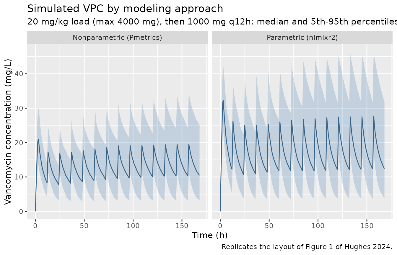
Replicates the layout of Figure 1 of Hughes 2024: simulated concentration-time percentiles for each modeling approach.
Steady-state exposure against the protocol AUC target
ss_start <- (n_days * 24) - tau   # last complete dosing interval

sim_ss <- sim |>
  dplyr::filter(!is.na(Cc)) |>
  dplyr::select(id, time, Cc, Approach)

conc_ss <- PKNCA::PKNCAconc(as.data.frame(sim_ss), Cc ~ time | Approach + id,
                            concu = "mg/L", timeu = "h")

dose_ss <- PKNCA::PKNCAdose(
  as.data.frame(events |> dplyr::filter(evid == 1) |> dplyr::select(id, time, amt)),
  amt ~ time | id, doseu = "mg")

int_ss <- data.frame(start = ss_start, end = ss_start + tau,
                     auclast = TRUE, cmax = TRUE, cmin = TRUE)

nca_ss <- PKNCA::pk.nca(PKNCA::PKNCAdata(conc_ss, dose_ss, intervals = int_ss))

ss_tbl <- as.data.frame(nca_ss$result) |>
  dplyr::filter(PPTESTCD == "auclast") |>
  # AUC over one 12 h interval at steady state -> daily AUC is twice that.
  mutate(auc24 = PPORRES * 24 / tau) |>
  group_by(Approach) |>
  summarise(`Median AUC0-24,ss (mg*h/L)` = median(auc24),
            `5th percentile` = quantile(auc24, 0.05),
            `95th percentile` = quantile(auc24, 0.95),
            `% in 400-600 target` = 100 * mean(auc24 >= 400 & auc24 <= 600),
            .groups = "drop")

knitr::kable(ss_tbl, digits = 1, caption = paste(
  "Steady-state daily exposure on the protocol regimen, by modeling approach.",
"The 400-600 mg*h/L window is the AUC target stated in Methods/Data Collection."))| Approach | Median AUC0-24,ss (mg*h/L) | 5th percentile | 95th percentile | % in 400-600 target |
|---|---|---|---|---|
| Nonparametric (Pmetrics) | 336.5 | 171.2 | 672.5 | 27.5 |
| Parametric (nlmixr2) | 455.1 | 234.1 | 940.7 | 34.5 |
# The paper's headline conclusion is that the two approaches agree clinically:
# "the clinical significance of these distributional differences seemed minimal".
# Assert on the MAGNITUDE of the median difference, not on its sign or on a bound
# taken from one draw -- both arms use common random numbers, but the cohort itself
# still varies with the solver thread count.
med <- ss_tbl$`Median AUC0-24,ss (mg*h/L)`
rel_diff <- 100 * abs(diff(med)) / mean(med)

# Realised ~25% here. The two models' typical clearances differ by 5.62 vs 4.37 L/h at
# the cohort median profile (a 25% exposure difference), which is a property of the
# published estimates, not of this draw. A 40% bound absorbs cohort noise while still
# going red if a parameter is mis-transcribed by a factor of 2 or a covariate term is
# dropped (either of which moves exposure by >= 80%).
stopifnot(rel_diff < 40)

# Both models must put the typical patient in a clinically plausible vancomycin range
# on this regimen -- an absolute sanity bound, not a race between the two arms.
stopifnot(all(med > 200), all(med < 900))
The two models place the median patient at different daily exposures on an identical regimen – the nonparametric model’s higher typical clearance (5.62 vs 4.37 L/h at the cohort median profile) translates into a correspondingly lower AUC. This is the practical face of the Figure 2 finding that “on an average, Pmetrics estimated higher values of CL and V than nlmixr2”. The paper judged the clinical significance of these distributional differences to be minimal, and reported near-identical individualized (a posteriori) predictive performance for the two approaches – nRMSE 13.8% versus 13.1%, MPE 0.16% versus 0.84% (Table 3) – which is the metric that matters for MIPD, where each patient’s parameters are updated from their own measured levels.
Model-fit statistics reported by the paper
For reference, these are the fit statistics from Table 3. They depend on the original patient-level dataset, which is not publicly available, so they cannot be recomputed here; they are reproduced only so the two packaged models can be read alongside the performance that motivated them.
tibble::tribble(
  ~Metric,                          ~`Parametric (nlmixr2)`, ~`Nonparametric (Pmetrics)`,
  "r^2, population (a priori)",     0.597,                   0.531,
  "r^2, individual (a posteriori)", 0.896,                   0.917,
  "MPE %, population",              26.3,                    2.69,
  "MPE %, individual",              0.16,                    0.84,
  "nRMSE %, population",            27.2,                    30.7,
  "nRMSE %, individual",            13.8,                    13.1
) |>
knitr::kable(caption = "Table 3 of Hughes 2024, model-fit rows (reproduced, not recomputed).")| Metric | Parametric (nlmixr2) | Nonparametric (Pmetrics) |
|---|---|---|
| r^2, population (a priori) | 0.597 | 0.531 |
| r^2, individual (a posteriori) | 0.896 | 0.917 |
| MPE %, population | 26.300 | 2.690 |
| MPE %, individual | 0.160 | 0.840 |
| nRMSE %, population | 27.200 | 30.700 |
| nRMSE %, individual | 13.800 | 13.100 |
Assumptions and deviations
-
Infusion duration is an assumption. The paper
states that vancomycin was given by intermittent infusion and that peaks
were drawn “within 2 h after the end of infusion”, but never states the
infusion duration. The simulations above infuse at 1000 mg/h, the
standard maximum vancomycin rate. This affects the shape of the peak but
not AUC, and the closed-form gate (
AUC0-inf = Dose/CL) is invariant to it. - Maintenance regimen is an assumption. The protocol individualized maintenance dosing to an AUC target rather than fixing a dose. A flat 1000 mg q12h is used here so that the two models are compared on an identical regimen; it is not a dose the paper recommends.
- Virtual-cohort distributional shapes are assumptions. Table 1 reports medians and ranges only, so the distributions (normal for height and age, shifted-lognormal for BMI, lognormal for serum creatinine) were chosen to reproduce those medians and ranges. Race and ethnicity were not reported and are not simulated.
-
Eta correlations are not encoded. The parametric
model was fitted with a correlated
BLOCK(3)on CL, Vc and Vp (SDC1 S3 declareseta_CL + eta_V + eta_V2 ~ c(...)), but the final off-diagonal estimates are published in neither the paper nor the supplement. Encoding them would mean inventing covariances, so both packaged models use independent etas. For scale, the NONMEM listing in SDC1 S4 implies correlations of 0.74 (CL-Vc), 0.12 (CL-Vp) and 0.66 (Vc-Vp), but those belong to a different parameter set (see Errata) and are not transferable to the nlmixr2 column. - The nonparametric joint density is not recoverable. NPAG’s output is a discrete distribution over support points, and its shape – including any multimodality, which is the main reason to run a nonparametric method at all – cannot be reconstructed from the published summary table. The packaged nonparametric model approximates each marginal as an independent lognormal matching the reported median and %CV. The Table 2 “Range” column spans the support points and is recorded in the parameter labels, but it is not an uncertainty interval and is not encoded as a variance. The Discussion itself notes that no subgroups could be identified in this analysis.
-
Pmetrics
lambdais not encoded. The nonparametric residual model is the assay polynomialSD = C0 + C1*CwithC0 = 0.5,C1 = 0.1(encoded viacombined1(), which is a linear sum, unlike nlmixr2’s default quadrature combination). Pmetrics additionally fits an additive noise term, reported asL = 0.1in Table 3 and the SDC1 S5#Errblock, which nlmixr2 has no direct analogue for. Omitting it makes the encoded residual SD a very slight underestimate: at 10 mg/L, 1.500 encoded against 1.503 in Pmetrics. -
BSV scale conventions differ between the two files,
deliberately. For the parametric model the reported “%CV” is
100*sqrt(omega^2), which is demonstrated by the paper’s own NONMEM$OMEGA BLOCK(3)reproducing the Table 2 NONMEM %CV row exactly (0.0473154, 0.0322236, 0.634656 -> 21.75 / 17.95 / 79.67 against a published 21.8 / 18.0 / 79.7; the exact lognormal conversion would give 22.0 / 18.1 / 94.1). For the nonparametric model the %CV is a genuine descriptive coefficient of variation of the discrete distribution, so the exact lognormal conversionomega^2 = log(CV^2 + 1)is used instead. Both are documented at the point of use in the model files. - No published NCA to compare against. Hughes 2024 reports no Cmax / Tmax / AUC / half-life table, so the NCA comparison above uses closed-form identities derived from the published parameters rather than a published NCA table.
Errata and internal inconsistencies in the source
-
The parametric residual error is reported three different
ways. Table 2’s nlmixr2 column gives a proportional error of
16.8% with the additive row shown as “-”; Table 3 gives “15.6% + 1.2
mg/L”; and the SDC1 S4 NONMEM listing gives
PROP = 0.157812withADD = 0.001. The 1.2 mg/L additive term in Table 3 appears nowhere else – not in Table 2, not in the S3 nlmixr2 code (which declaresadd_sd <- fixed(1e-3)), not in S4. The packaged model uses Table 2’s 16.8% with the additive fixed at 0.001 mg/L, because Table 2 is the paper’s dedicated parameter-estimate table and its nlmixr2 column is the model being encoded, and because both supplement listings agree that the additive term is a nominal fixed value rather than an estimated 1.2 mg/L. -
SDC1 S4 is labelled “NONMEM with final estimates” but does
not match Table 2’s NONMEM column. S4 gives CL 5.21846, V1
65.1888, Q 6.65364, V2 62.6624,
THETA(8)0.859415, and an$OMEGA BLOCK(3)whose diagonal is 0.0635929 / 0.0631089 / 0.520521 (25.2 / 25.1 / 72.2 %CV). Table 2’s NONMEM column gives CL 5.06, Vc 64.34, Q 6.24, Vp 59.0, u3 0.851 and BSV 21.8 / 18.0 / 79.7 %CV. The Table 2 values are the ones reproduced by the Hughes control stream published in the Tong 2026 supplement (modellib("Tong_2026_vancomycin_hughes"): 5.0627, 64.339, 6.2402, 59.019, 0.8509), so S4 appears to be an earlier or otherwise different run. Neither S4 nor the Table 2 NONMEM column is packaged from this paper; the NONMEM parameter set already exists in the library via the Tong 2026 extraction. -
SDC1 S3 lists initial estimates, not final ones.
The nlmixr2 code block declares
tCL <- log(3),tV <- log(60),tQ <- log(2),tV2 <- log(100),tCRCL_CL <- 0.5and unit-variance etas – starting values, not the fitted results. It is used here only to establish model structure (which parameters are estimated, which are fixed, the residual-error form and theBLOCK(3)eta structure); every value comes from Table 2. -
SDC1 S5 lists
TH1, 0.5in the Pmetrics#Priblock, which is a prior specification (a search range or starting value), not the fitted estimate. Table 2 reports the fittedu3as 1.05 with 10% RSE, and that is what is encoded. -
The Table 2 footnote’s
u1allometric exponent is not in either final model – see the note under the Source trace table above.