Nicotine intravenous, oral, buccal and transdermal (Olsson Gisleskog 2021)

Model and source

Olsson Gisleskog et al. (2021) pooled 29 single- and repeated-dose studies of Nicorette and related nicotine replacement products in 930 healthy smokers and fitted seven population PK models: one for intravenous nicotine and one each for oral microtablets, mouth spray, chewing gum, lozenge, inhaler and transdermal patch. Joint fits across routes did not converge, so the intravenous model was fitted first and its disposition parameters and their between-subject variability were then held fixed in the six extravascular models. The library follows the same structure: seven model files, all described in this article.

• Citation: Olsson Gisleskog PO, Perez Ruixo JJ, Westin A, Hansson AC, Soons PA. Nicotine Population Pharmacokinetics in Healthy Smokers After Intravenous, Oral, Buccal and Transdermal Administration. Clin Pharmacokinet. 2021;60(4):541-561. doi:10.1007/s40262-020-00960-5
• Article: https://doi.org/10.1007/s40262-020-00960-5 (open access)
• Supplementary NONMEM control streams and output for all seven final models (Electronic Supplementary Material 7): https://static-content.springer.com/esm/art%3A10.1007%2Fs40262-020-00960-5/MediaObjects/40262_2020_960_MOESM7_ESM.docx

model_names <- c(
  iv = "OlssonGisleskog_2021_nicotine_iv",
  oral = "OlssonGisleskog_2021_nicotine_oral",
  mouthspray = "OlssonGisleskog_2021_nicotine_mouthspray",
  gum = "OlssonGisleskog_2021_nicotine_gum",
  lozenge = "OlssonGisleskog_2021_nicotine_lozenge",
  inhaler = "OlssonGisleskog_2021_nicotine_inhaler",
  transdermal = "OlssonGisleskog_2021_nicotine_transdermal"
)
mods <- lapply(model_names, function(n) rxode2::rxode(readModelDb(n)))
#> ℹ parameter labels from comments will be replaced by 'label()'
#> ℹ parameter labels from comments will be replaced by 'label()'
#> ℹ parameter labels from comments will be replaced by 'label()'
#> Warning: some etas defaulted to non-mu referenced, possible parsing error: etaiov_ktr_6, etaiov_ktr_5, etaiov_ktr_4, etaiov_ktr_3, etaiov_ktr_2, etaiov_ktr_1, etaiov_fsw_6, etaiov_fsw_5, etaiov_fsw_4, etaiov_fsw_3, etaiov_fsw_2, etaiov_fsw_1, etaiov_ka_6, etaiov_ka_5, etaiov_ka_4, etaiov_ka_3, etaiov_ka_2, etaiov_ka_1, etaiov_fcentral_6, etaiov_fcentral_5, etaiov_fcentral_4, etaiov_fcentral_3, etaiov_fcentral_2, etaiov_fcentral_1
#> as a work-around try putting the mu-referenced expression on a simple line
#> ℹ parameter labels from comments will be replaced by 'label()'
#> Warning: some etas defaulted to non-mu referenced, possible parsing error: etaiov_fcentral_5, etaiov_fcentral_4, etaiov_fcentral_3, etaiov_fcentral_2, etaiov_fcentral_1, etaiov_fsw_5, etaiov_fsw_4, etaiov_fsw_3, etaiov_fsw_2, etaiov_fsw_1
#> as a work-around try putting the mu-referenced expression on a simple line
#> ℹ parameter labels from comments will be replaced by 'label()'
#> Warning: some etas defaulted to non-mu referenced, possible parsing error: etaiov_ktr_5, etaiov_ktr_4, etaiov_ktr_3, etaiov_ktr_2, etaiov_ktr_1, etaiov_krel_5, etaiov_krel_4, etaiov_krel_3, etaiov_krel_2, etaiov_krel_1, etaiov_fsw_5, etaiov_fsw_4, etaiov_fsw_3, etaiov_fsw_2, etaiov_fsw_1, etaiov_fcentral_5, etaiov_fcentral_4, etaiov_fcentral_3, etaiov_fcentral_2, etaiov_fcentral_1
#> as a work-around try putting the mu-referenced expression on a simple line
#> ℹ parameter labels from comments will be replaced by 'label()'
#> Warning: some etas defaulted to non-mu referenced, possible parsing error: etaiov_ktr_2, etaiov_ktr_1, etaiov_fsw_2, etaiov_fsw_1, etaiov_fcentral_2, etaiov_fcentral_1
#> as a work-around try putting the mu-referenced expression on a simple line
#> ℹ parameter labels from comments will be replaced by 'label()'
#> Warning: some etas defaulted to non-mu referenced, possible parsing error: etaiov_fdepot_6, etaiov_fdepot_5, etaiov_fdepot_4, etaiov_fdepot_3, etaiov_fdepot_2, etaiov_fdepot_1, etaiov_fcentral_6, etaiov_fcentral_5, etaiov_fcentral_4, etaiov_fcentral_3, etaiov_fcentral_2, etaiov_fcentral_1
#> as a work-around try putting the mu-referenced expression on a simple line

# Every model must be integrated as written: a cl/vc pair must not have been
# turned into an analytic linCmt() solution that would drop the absorption
# chains.
stopifnot(all(vapply(mods, function(m) is.null(m$linCmt), logical(1))))

tibble(
  Model = unname(model_names),
  Description = vapply(mods, function(m) m$description, character(1))
) |>
  knitr::kable()

Model	Description
OlssonGisleskog_2021_nicotine_iv	Three-compartment population PK model for intravenous nicotine in healthy adult smokers (Olsson Gisleskog 2021; 80 subjects, 4 studies, 0.028 mg/kg infused over 10 min). Clearance and inter-compartmental flows are allometrically scaled by (WT/70)^0.75 and the three volumes by (WT/70)^1. Residual nicotine from pre-study smoking is described by a virtual 1-mg bolus into the central compartment at the start of the 36-h washout, whose bioavailability (the pre-washout nicotine dose, 4.90 mg) carries its own IIV; the record is flagged with VIRTUAL_DOSE = 1. This IV model supplies the disposition parameters (and their IIV) that the paper’s oral, buccal and transdermal models hold fixed.
OlssonGisleskog_2021_nicotine_oral	Population PK model for orally ingested nicotine microtablets in healthy adult smokers (Olsson Gisleskog 2021; 26 subjects, 2 studies, 2 and 6 mg). Disposition (three compartments with allometric weight scaling) and its IIV are fixed to the paper’s intravenous model. Absorption differs by study: in 92NNBT005 (repeated dosing, tablets chewed) first-order absorption directly into the central compartment (ka 1.55 1/h, F 39.5%); in 93NNBT007 (single dose, tablets swallowed whole) first-order transfer at the same ka into a chain of three transit compartments (ktr 3.60 1/h, F 22.3%). A transient time-dependent increase in clearance during the repeated-dose day (77.3% maximum, 50% onset at 5.29 h after the first dose, lasting 1.92 h) applies in 92NNBT005 only. Residual pre-study nicotine is a virtual 1-mg bolus into central at the start of the washout with bioavailability 4.92 mg.
OlssonGisleskog_2021_nicotine_mouthspray	Population PK model for nicotine oromucosal mouth spray (Nicorette QuickMist, 1 mg per spray) in healthy adult smokers (Olsson Gisleskog 2021; 201 subjects, 6 studies, 1-4 mg). Disposition (three compartments with allometric weight scaling) and its IIV are fixed to the paper’s intravenous model. The dose is delivered as a bolus split between the buccal cavity and the gut: a dose-dependent fraction Frsw (60.6% at 2 mg, rising with dose, logit-scale IOV) is swallowed and absorbed through a gut compartment and two transit compartments (ktr 3.70 1/h) with oral bioavailability fixed to 39.5%; the remainder is absorbed oromucosally (F = 1) after a 1.4-min lag with ka 15.9 1/h (buccal spraying) or 86.0 1/h (sublingual spraying). A transient time-dependent clearance increase (35.7% maximum) describes the lower-than-expected accumulation on repeated dosing. Residual pre-study nicotine is a virtual 1-mg bolus into central at the start of the washout (bioavailability 4.84 mg). IOV over up to six study periods on ka, Frsw, ktr and the pre-washout dose.
OlssonGisleskog_2021_nicotine_gum	Population PK model for nicotine chewing gum (Nicorette classic and Freshmint/Freshfruit coated gum, 2-6 mg, chewed for 30 min) in healthy adult smokers (Olsson Gisleskog 2021; 512 subjects, 14 studies). Disposition (three compartments with allometric weight scaling) and its IIV are fixed to the paper’s intravenous model. Nicotine is released from the gum by a first-order process whose rate is calculated from the individual amount released, and release stops at the end of the 0.5-h chewing period. A fraction Frsw (54.7%, logit-scale IOV) of the dose is swallowed, released at the same rate in the gut and absorbed through three transit compartments (ktr 5.53 1/h) with oral bioavailability fixed to 39.5%; the remainder passes from the gum to the buccal cavity after a lag and is absorbed oromucosally (F = 1) with ka 26.5 1/h (Nicorette classic) or 9.29 1/h (Freshmint/Freshfruit) at 2 mg, scaled by (dose/2)^0.507. On repeated dosing a transient time-dependent decrease in oral bioavailability (75.2% maximum, logit-scale IIV) describes the lower-than-expected accumulation. Residual pre-study nicotine is a virtual 1-mg bolus into central at the start of the washout (bioavailability 6.93 mg).
OlssonGisleskog_2021_nicotine_lozenge	Population PK model for nicotine lozenges (Nicorette and NiQuitin, 2 and 4 mg, dissolved in the mouth) in healthy adult smokers (Olsson Gisleskog 2021; 303 subjects, 6 studies). Disposition (three compartments with allometric weight scaling) and its IIV are fixed to the paper’s intravenous model. Nicotine is released from the lozenge by a first-order process (Krel 6.41 1/h, IOV). A fraction Frsw of the dose is swallowed (68.8% for 4-mg NiQuitin, lower at 2 mg and higher for Nicorette lozenges; logit-scale IOV), released at the same rate in the gut and absorbed through three transit compartments (ktr 3.54 1/h, IOV) with oral bioavailability fixed to 39.5%; the remainder passes after a lag into the buccal cavity and is absorbed oromucosally (ka 11.6 1/h, F = 1 with IIV). A transient time-dependent clearance increase (54.4% maximum) describes the lower-than-expected accumulation on repeated dosing. Residual pre-study nicotine is a virtual 1-mg bolus into central at the start of the washout (bioavailability 5.44 mg).
OlssonGisleskog_2021_nicotine_inhaler	Population PK model for the nicotine inhaler (Nicorette Inhalator, 10 and 15 mg cartridges, inhaled over 20-min sessions) in healthy adult smokers (Olsson Gisleskog 2021; 58 subjects, 3 studies). Disposition (three compartments with allometric weight scaling) and its IIV are fixed to the paper’s intravenous model. The amount released per session (from the inhaler weight change) enters as a 20-min zero-order input split between the buccal cavity and the gut: a fraction Frsw (66.9%, logit-scale IOV) is swallowed and absorbed through a gut compartment and two transit compartments (ktr 5.26 1/h, IOV) with oral bioavailability fixed to 39.5%; the remainder is absorbed oromucosally (ka 0.753 1/h, F = 1 with IIV). Bioavailability of both routes is 66% higher in study 97NNIN024. A transient time-dependent clearance increase (23.2% maximum, IIV) describes the lower-than-expected accumulation on repeated dosing. Residual pre-study nicotine is a virtual 1-mg bolus into central at the start of the washout (bioavailability 7.31 mg).
OlssonGisleskog_2021_nicotine_transdermal	Population PK model for transdermal nicotine patches (Nicorette patch 5-15 mg/16 h and Nicorette Invisipatch 10-25 mg/16 h, worn 16 or 24 h) in healthy adult smokers (Olsson Gisleskog 2021; 73 subjects, 3 studies). Disposition (three compartments with allometric weight scaling) and its IIV are fixed to the paper’s intravenous model. Nicotine leaves the patch by two parallel pathways: a fraction Fr1 (40.0% Nicorette patch, 71.9% Invisipatch; logit-scale IIV) by a first-order release (Krel 0.146 1/h) that runs from application (after a 0.53-h lag for Invisipatch) for a fraction Frdur1 of 16 h (44.5% and 96.2%), scaled so that the whole fraction is delivered in that window, and the remainder by a zero-order release from 4.06 h after application until patch removal. Released nicotine is absorbed through three transit compartments (ktr 3.62 1/h) with transdermal bioavailability 75.8% (IOV). Clearance is 11.6% higher from 25 h after the first application. Residual pre-study nicotine is a virtual 1-mg bolus into central at the start of the washout (bioavailability 3.82 mg).

All models share the same disposition: three compartments with clearance and inter-compartmental flows scaled by (WT/70)^0.75 and volumes by (WT/70)^1. Concentrations are in ng/mL, doses in mg and time in hours.

Every model also carries the paper’s device for residual nicotine from smoking before the study: a virtual bolus of 1 mg given into central at the start of the washout, whose bioavailability fcentral (reported as the “pre-washout nicotine dose”, 3.8-7.3 mg across models) has its own IIV and, where there were several periods, IOV. In the extravascular models only this virtual dose enters central. In the intravenous model the real infusion also enters central, so the virtual-dose record is flagged with VIRTUAL_DOSE = 1. Omit the virtual dose to simulate a subject with no residual nicotine; this article does so except where a published figure shows the washout.

Population

pop <- lapply(mods, function(m) m$population)
tibble(
  Model = names(pop),
  N = vapply(pop, function(p) p$n_subjects, integer(1)),
  Studies = vapply(pop, function(p) p$n_studies, integer(1)),
  `Age, median (range)` = paste0(vapply(pop, function(p) p$age_median, character(1)), " (", vapply(pop, function(p) p$age_range, character(1)), ")"),
  `Weight, median (range)` = paste0(vapply(pop, function(p) p$weight_median, character(1)), " (", vapply(pop, function(p) p$weight_range, character(1)), ")"),
  `Female (%)` = vapply(pop, function(p) p$sex_female_pct, numeric(1)),
  Doses = vapply(pop, function(p) p$dose_range, character(1))
) |>
  knitr::kable(caption = "Study populations by model (Olsson Gisleskog 2021 Tables 1 and 2).")

Study populations by model (Olsson Gisleskog 2021 Tables 1 and 2).

Model	N	Studies	Age, median (range)	Weight, median (range)	Female (%)	Doses
iv	80	4	36 years (20-76 years)	72.9 kg (49.0-99.0 kg)	46.2	0.028 mg/kg nicotine intravenous infusion over 10 min
oral	26	2	38 years (24-47 years)	62.5 kg (44.0-105.0 kg)	53.8	2 and 6 mg nicotine microtablets, single (93NNBT007) and repeated (92NNBT005) oral doses
mouthspray	201	6	27 years (18-50 years)	72.6 kg (49.4-105.6 kg)	44.3	1, 2, 3 and 4 mg nicotine oromucosal spray, single and repeated doses
gum	512	14	26 years (18-50 years)	71.5 kg (40.6-108.0 kg)	48.0	2, 4 and 6 mg nicotine chewing gum chewed for 30 min, single and repeated doses
lozenge	303	6	28 years (18-50 years)	72.8 kg (52.2-105.0 kg)	47.2	2 and 4 mg nicotine lozenge (Nicorette, NiQuitin), single and repeated doses
inhaler	58	3	29 years (22-49 years)	71.0 kg (43.0-101.0 kg)	53.4	Nicotine inhaler, about 2 mg released per 20-min inhalation session, single and repeated sessions
transdermal	73	3	24 years (19-50 years)	71.2 kg (43.2-112.8 kg)	38.4	5, 10, 15, 25 and 37 mg nicotine patches applied for 16 h (24 h in one arm), single and three daily applications

All subjects were healthy adult smokers (typically 15-20 cigarettes/day), almost all White, studied at clinical units in Sweden between 1993 and 2012. The intravenous dataset excluded subjects with hepatic or renal impairment. Demographics were similar across routes, with slightly older subjects in the intravenous and oral studies. No covariate other than body weight (as fixed allometry) was retained in any model.

Source trace

Every ini() value carries an in-file comment naming its source: Tables 3-6 of the paper and the final NONMEM control streams and output files in the electronic supplementary material (ESM). The table below is generated from those comments so that it cannot drift from the model files. The disposition parameters and their IIV are the same fixed values in all six extravascular models; they are listed once, under the intravenous model, and checked for identity in code below.

# Parse the ini() block of a model file into (parameter, value, source) rows.
# Assignment lines are followed by a label() line that carries the source
# comment; eta lines carry it on the same line (or on the closing line of a
# multi-line block).
trace_ini <- function(file) {
  x <- readLines(file)
  start <- grep("^\\s*ini\\(\\{", x)
  end <- grep("^\\s*\\}\\)", x)
  end <- end[end > start][1]
  x <- x[(start + 1):(end - 1)]
  rows <- list()
  cur <- NULL
  eta_lhs <- NULL
  eta_rhs <- ""
  for (ln in x) {
    has_cmt <- grepl("#", ln)
    code <- trimws(sub("#.*$", "", ln))
    cmt <- if (has_cmt) trimws(sub("^[^#]*#", "", ln)) else ""
    if (!is.null(eta_lhs)) {
      eta_rhs <- paste(eta_rhs, code)
      if (has_cmt) {
        rows[[length(rows) + 1]] <- c(eta_lhs, eta_rhs, cmt)
        eta_lhs <- NULL
      }
    } else if (grepl("^[A-Za-z][A-Za-z0-9_.]*\\s*<-", code)) {
      cur <- c(trimws(sub("<-.*$", "", code)), trimws(sub("^[^<]*<-", "", code)))
    } else if (grepl("^label\\(", code) && !is.null(cur)) {
      rows[[length(rows) + 1]] <- c(cur, cmt)
      cur <- NULL
    } else if (grepl("~", code)) {
      lhs <- trimws(sub("~.*$", "", code))
      rhs <- trimws(sub("^[^~]*~", "", code))
      if (has_cmt) {
        rows[[length(rows) + 1]] <- c(lhs, rhs, cmt)
      } else {
        eta_lhs <- lhs
        eta_rhs <- rhs
      }
    }
  }
  out <- as.data.frame(do.call(rbind, rows), stringsAsFactors = FALSE)
  names(out) <- c("parameter", "value", "source")
  out
}

model_file <- function(n) {
  f <- system.file("modeldb", "specificDrugs", paste0(n, ".R"), package = "nlmixr2lib")
  if (!nzchar(f)) stop("model file not found for ", n)
  f
}

trace <- bind_rows(lapply(names(model_names), function(k) {
  trace_ini(model_file(model_names[[k]])) |> mutate(model = k, .before = 1)
}))

# Every ini() entry of every model must have been captured with a source.
n_ini <- vapply(mods, function(m) {
  d <- m$iniDf
  # a block of correlated etas is one source row; count its diagonal entries
  # as one row per block
  n_theta <- sum(!is.na(d$ntheta))
  etas <- d[is.na(d$ntheta), ]
  diag_rows <- etas[etas$neta1 == etas$neta2, ]
  in_block <- diag_rows$neta1 %in% c(etas$neta1[etas$neta1 != etas$neta2], etas$neta2[etas$neta1 != etas$neta2])
  n_theta + sum(!in_block) + as.integer(any(in_block))
}, integer(1))
n_trace <- table(factor(trace$model, levels = names(model_names)))
stopifnot(identical(as.integer(n_trace), unname(n_ini)))
stopifnot(all(nzchar(trace$source)))

shared <- c("lcl", "lvc", "lq", "lvp", "lq2", "lvp2", "e_wt_cl_q", "e_wt_vc_vp")
ev_models <- setdiff(names(mods), "iv")
iv_ini <- mods$iv$iniDf
for (k in ev_models) {
  d <- mods[[k]]$iniDf
  # Disposition thetas: same values as the IV estimates, and fixed.
  stopifnot(
    isTRUE(all.equal(d$est[match(shared, d$name)], iv_ini$est[match(shared, iv_ini$name)])),
    all(d$fix[match(shared, d$name)])
  )
  # Disposition IIV (CL and the V1/V3/V2 block): same values, fixed.
  eta_names <- c("etalcl", "etalvc", "etalvp2", "etalvp")
  iv_om <- mods$iv$omega[eta_names, eta_names]
  om <- mods[[k]]$omega[eta_names, eta_names]
  stopifnot(isTRUE(all.equal(unname(om), unname(iv_om))))
}

trace |>
  filter(model == "iv" | !(parameter %in% c(shared, "etalcl", "etalvc + etalvp2 + etalvp"))) |>
  rename(Model = model, Parameter = parameter, `Value (as coded)` = value, Source = source) |>
  knitr::kable(caption = "Source of every ini() value (ESM = electronic supplementary material, NONMEM code and output).")

Source of every ini() value (ESM = electronic supplementary material, NONMEM code and output).

Model	Parameter	Value (as coded)	Source
iv	lcl	log(67.4136)	Table 3 ‘CL (L/h)’ 67.4; ESM $THETA 67.4136
iv	lvc	log(117.373)	Table 3 ‘V1 (L)’ 117; ESM $THETA 117.373
iv	lq	log(38.615)	Table 3 ‘Q2 (L/h)’ 38.6; ESM $THETA 38.615
iv	lvp	log(130.372)	Table 3 ‘V2 (L)’ 130; ESM $THETA 130.372
iv	lq2	log(216.29)	Table 3 ‘Q3 (L/h)’ 216; ESM $THETA 216.29
iv	lvp2	log(53.4189)	Table 3 ‘V3 (L)’ 53.4; ESM $THETA 53.4189
iv	e_wt_cl_q	fixed(0.75)	Sect. 2.3.1 ‘allometric exponent for CL and intercompartmental flows was fixed to 0.75’
iv	e_wt_vc_vp	fixed(1)	Sect. 2.3.1 ‘and to 1.0 for Vn’
iv	lfcentral	log(4.90)	Table 3 ‘Pre-washout nicotine dose (mg)’ 4.90; ESM output TH7 4.90E+00
iv	etalcl	0.0705245	Table 3 ‘IIV CL’ 27.0% CV; ESM $OMEGA IIV_CL 0.0705245
iv	etalvc + etalvp2 + etalvp	c( 0.381077, -0.230826, 0.450311, 0, 0.5527, 1.83554 )	Table 3 IIV V1 68.1%, IIV V3 75.4%, IIV V2 230%, covariances V1/V3 -0.231 and V2/V3 0.553; ESM $OMEGA BLOCK(3)
iv	etalfcentral	0.519	Table 3 ‘IIV pre washout nicotine dose’ 82.5% CV; ESM output OMEGA(5,5) 5.19E-01
iv	propSd	0.0926	Table 3 ‘Proportional residual error’ 0.0926
iv	addSd	0.212	Table 3 ‘Additive residual error (ng/mL)’ 0.212
oral	lka	log(1.55)	Table 4 ‘Ka (h-1)’ 1.55
oral	lfdepot_92nnbt005	log(0.395)	Table 4 ‘F study 92NNBT005 (%)’ 39.5
oral	lfdepot_93nnbt007	log(0.223)	Table 4 ‘F study 93NNBT007 (%)’ 22.3
oral	lktr	log(3.60)	Table 4 ‘Ktr study 93NNBT007 (h-1)’ 3.60
oral	lcl_t50	log(5.29)	Table 4 ‘Start (h)’ 5.29
oral	lcl_time_dur	log(1.92)	Table 4 ‘Duration (h)’ 1.92
oral	lcl_time_max	log(0.773)	Table 4 ‘Emax (%)’ 77.3
oral	lcl_time_hill	log(12.3)	Table 4 ‘pow’ 12.3
oral	lfcentral	log(4.92)	Table 4 ‘Pre-washout nicotine dose (mg)’ 4.92
oral	etalfdepot	0.0499	Table 4 ‘IIV F’ 22.6% CV; ESM output OMEGA(5,5) 4.99E-02
oral	etalktr	0.186	Table 4 ‘IIV Ktr’ 45.2% CV; ESM output OMEGA(6,6) 1.86E-01
oral	etalfcentral	0.610	Table 4 ‘IIV pre-washout nicotine dose’ 91.7% CV; ESM output OMEGA(7,7) 6.10E-01
oral	etalcl_time_dur	0.340	Table 4 ‘IIV duration’ 63.7% CV; ESM output OMEGA(8,8) 3.40E-01
oral	propSd	0.0987	Table 4 ‘Proportional residual error (%)’ 9.87
oral	addSd	0.162	Table 4 ‘Additive residual error (ng/mL)’ 0.162
mouthspray	lka_buccal	log(15.9)	Table 5 ‘Ka (h-1)’ 15.9 (footnote c, buccal)
mouthspray	lka_sublingual	log(86.0)	Table 5 ‘Ka (h-1)’ 86.0 (footnote c, sublingual)
mouthspray	ltlag	log(0.0230)	Table 5 ‘Lag time (h)’ 0.0230
mouthspray	logitfsw	logit(0.606)	Table 5 ‘Frsw (%)’ 60.6 at 2 mg (footnote e); ESM output TH10 0.606
mouthspray	e_dose_nicotine_mg_fsw	0.0928	ESM output TH11 9.28E-02 (POWFRSW); reproduces Table 5 Frsw 64.6% at 4 mg
mouthspray	lktr	log(3.70)	Table 5 ‘Ktrg (h-1)’ 3.70
mouthspray	lfdepot_buccal	fixed(log(1))	ESM $THETA ‘1 FIX ; F total’; Sect. 2.3.4 ‘a F of 100%’
mouthspray	lfdepot_oral	fixed(log(0.395))	ESM $PK ORAL_F = 0.395*EXP(ETA(6)); Table 4 F study 92NNBT005 39.5|mouthspray |lcl_t50 |log(3.37) |Table 5 'Start (h)' 3.37 | |mouthspray |lcl_time_dur |log(8.78) |Table 5 'Duration (h)' 8.78 | |mouthspray |lcl_time_max |log(0.357) |Table 5 'Emax (|mouthspray |lcl_time_hill |log(4.82) |Table 5 'pow' 4.82 | |mouthspray |lfcentral |log(4.84) |Table 5 'Pre-washout nicotine dose (mg)' 4.84 | |mouthspray |etaltlag |0.0472 |Table 5 'IIV lag time' 22.0|mouthspray |etalfdepot_oral |0.307 |Table 5 'IIV Foral' 60.0|mouthspray |etalfcentral |0.509 |Table 5 'IIV pre-washout nicotine dose' 81.5|mouthspray |etalcl_time_dur |0.543 |Table 5 'IIV duration' 84.9|mouthspray |etaiov_fcentral_1 |0.229 |Table 5 'IOV pre-washout nicotine dose' 50.7|mouthspray |etaiov_fcentral_2 |fixed(0.229) |$OMEGA BLOCK(1) SAME
mouthspray	etaiov_fcentral_3	fixed(0.229)	$OMEGA BLOCK(1) SAME | |mouthspray |etaiov_fcentral_4 |fixed(0.229) |$OMEGA BLOCK(1) SAME
mouthspray	etaiov_fcentral_5	fixed(0.229)	$OMEGA BLOCK(1) SAME | |mouthspray |etaiov_fcentral_6 |fixed(0.229) |$OMEGA BLOCK(1) SAME
mouthspray	etaiov_ka_1	0.653	Table 5 ‘IOV Ka’ 96.0% CV; ESM output OMEGA(15,15) 6.53E-01
mouthspray	etaiov_ka_2	fixed(0.653)	$OMEGA BLOCK(1) SAME | |mouthspray |etaiov_ka_3 |fixed(0.653) |$OMEGA BLOCK(1) SAME
mouthspray	etaiov_ka_4	fixed(0.653)	$OMEGA BLOCK(1) SAME | |mouthspray |etaiov_ka_5 |fixed(0.653) |$OMEGA BLOCK(1) SAME
mouthspray	etaiov_ka_6	fixed(0.653)	$OMEGA BLOCK(1) SAME | |mouthspray |etaiov_fsw_1 |0.294 |Table 5 'IOV Frsw' 0.294 (logit scale); ESM output OMEGA(21,21) 2.94E-01 | |mouthspray |etaiov_fsw_2 |fixed(0.294) |$OMEGA BLOCK(1) SAME
mouthspray	etaiov_fsw_3	fixed(0.294)	$OMEGA BLOCK(1) SAME | |mouthspray |etaiov_fsw_4 |fixed(0.294) |$OMEGA BLOCK(1) SAME
mouthspray	etaiov_fsw_5	fixed(0.294)	$OMEGA BLOCK(1) SAME | |mouthspray |etaiov_fsw_6 |fixed(0.294) |$OMEGA BLOCK(1) SAME
mouthspray	etaiov_ktr_1	0.353	Table 5 ‘IOV Ktr’ 65.1% CV; ESM output OMEGA(27,27) 3.53E-01
mouthspray	etaiov_ktr_2	fixed(0.353)	$OMEGA BLOCK(1) SAME | |mouthspray |etaiov_ktr_3 |fixed(0.353) |$OMEGA BLOCK(1) SAME
mouthspray	etaiov_ktr_4	fixed(0.353)	$OMEGA BLOCK(1) SAME | |mouthspray |etaiov_ktr_5 |fixed(0.353) |$OMEGA BLOCK(1) SAME
mouthspray	etaiov_ktr_6	fixed(0.353)	$OMEGA BLOCK(1) SAME
mouthspray	propSd	0.101	Table 5 ‘Proportional residual error (%)’ 10.1
mouthspray	addSd	0.136	Table 5 (continued) ‘Additive residual error (ng/mL)’ 0.136
gum	ltlag	log(0.0531)	Table 5 ‘Lag time (h)’ 0.0531
gum	lka_classic	log(26.5)	Table 5 ‘Ka (h-1)’ 26.5 (footnote d); ESM $PK TVKA reference NDOSE/2
gum	lka_freshmint	log(9.29)	Table 5 ‘Ka (h-1)’ 9.29 (footnote d)
gum	e_dose_nicotine_mg_ka	0.507	Table 5 ‘Dose on Ka’ 0.507; ESM TVKA = …*(NDOSE/2)**POWKA
gum	logitfsw	logit(0.547)	Table 5 ‘Frsw (%)’ 54.7
gum	lktr	log(5.53)	Table 5 ‘Ktrg (h-1)’ 5.53
gum	lfdepot_buccal	fixed(log(1))	ESM $PK TVFBUCC = 1; Sect. 2.3.4 ‘a F of 100%’
gum	lfdepot_oral	fixed(log(0.395))	ESM $PK TVORAL_F = 0.395; Table 4 F study 92NNBT005 39.5|gum |logitfdepot_oral_time_max |logit(0.752) |Table 5 'Emax (|gum |lfdepot_oral_t50 |log(0.636) |Table 5 'Start (h)' 0.636 | |gum |lfdepot_oral_time_dur |log(13.9) |Table 5 'Duration (h)' 13.9 | |gum |fdepot_oral_time_hill |6.75 |Table 5 'pow' 6.75 | |gum |lfcentral |log(6.93) |Table 5 'Pre-washout nicotine dose (mg)' 6.93 | |gum |etaltlag |0.132 |Table 5 'IIV lag time' 37.5|gum |etalfdepot_oral |0.411 |Table 5 'IIV Foral' 71.3|gum |etalogitfdepot_oral_time_max |2.67 |Table 5 'IIV Emax' 366 (logit-scale variance printed through the CV formula); ESM output OMEGA(7,7) 2.67E+00 | |gum |etalfdepot_oral_t50 |0.275 |Table 5 'IIV start' 56.3|gum |etalfdepot_oral_time_dur |0.537 |Table 5 'IIV duration' 84.3|gum |etalfcentral |0.549 |Table 5 'IIV pre-washout nicotine dose' 85.5|gum |etaiov_fsw_1 |1.04 |Table 5 'IOV Frsw' 1.04 (logit scale); ESM output OMEGA(11,11) 1.04E+00 | |gum |etaiov_fsw_2 |fixed(1.04) |$OMEGA BLOCK(1) SAME
gum	etaiov_fsw_3	fixed(1.04)	$OMEGA BLOCK(1) SAME | |gum |etaiov_fsw_4 |fixed(1.04) |$OMEGA BLOCK(1) SAME
gum	etaiov_fsw_5	fixed(1.04)	$OMEGA BLOCK(1) SAME | |gum |etaiov_fcentral_1 |0.164 |Table 5 'IOV pre-washout nicotine dose' 42.2|gum |etaiov_fcentral_2 |fixed(0.164) |$OMEGA BLOCK(1) SAME
gum	etaiov_fcentral_3	fixed(0.164)	$OMEGA BLOCK(1) SAME | |gum |etaiov_fcentral_4 |fixed(0.164) |$OMEGA BLOCK(1) SAME
gum	etaiov_fcentral_5	fixed(0.164)	$OMEGA BLOCK(1) SAME
gum	propSd	0.104	Table 5 ‘Proportional residual error (%)’ 10.4
gum	addSd	0.157	Table 5 (continued) ‘Additive residual error (ng/mL)’ 0.157
lozenge	lkrel	log(6.41)	Table 5 ‘Krel (h-1)’ 6.41
lozenge	ltlag	log(0.0437)	Table 5 ‘Lag time (h)’ 0.0437
lozenge	lka	log(11.6)	Table 5 ‘Ka (h-1)’ 11.6
lozenge	logitfsw	logit(0.688)	Table 5 ‘Frsw (%)’ 68.8 at 4 mg (footnote e); ESM output TH10 0.688
lozenge	e_form_nicotine_nicorette_lozenge_fsw	0.412	Table 5 ‘Nicorette on Frsw’ 0.412 (footnote g, additive on logit scale)
lozenge	e_dose2mg_fsw	-0.217	ESM output TH14 -2.17E-01; reproduces Table 5 Frsw 64.0% at 2 mg
lozenge	lktr	log(3.54)	Table 5 ‘Ktrg (h-1)’ 3.54
lozenge	lfdepot_buccal	fixed(log(1))	ESM $PK TVFBUCC = 1 with IIV; Sect. 2.3.4 ‘a F of 100%’
lozenge	lfdepot_oral	fixed(log(0.395))	ESM $PK ORAL_F = 0.395*EXP(ETA(7)); Table 4 F study 92NNBT005 39.5|lozenge |lcl_t50 |log(4.86) |Table 5 'Start (h)' 4.86 | |lozenge |lcl_time_dur |log(7.18) |ESM output TH17 7.18E+00 (SE 1.45, RSE 20.2|lozenge |lcl_time_max |log(0.544) |Table 5 'Emax (|lozenge |lcl_time_hill |log(3.18) |ESM output TH18 3.18E+00 (SE 0.314, RSE 9.87|lozenge |lfcentral |log(5.44) |Table 5 'Pre-washout nicotine dose (mg)' 5.44 | |lozenge |etaltlag |0.0991 |Table 5 'IIV lag time' 32.3|lozenge |etalka |0.637 |Table 5 'IIV Ka' 94.4|lozenge |etalfdepot_oral |0.316 |Table 5 'IIV Foral' 61.0|lozenge |etalfcentral |0.320 |Table 5 'IIV pre-washout nicotine dose' 61.4|lozenge |etalfdepot_buccal |0.0533 |Table 5 'IIV Fbuccal' 23.4|lozenge |etalcl_t50 |0.171 |Table 5 'IIV start' 43.2|lozenge |etalcl_time_dur |0.428 |Table 5 'IIV duration' 73.1|lozenge |etaiov_fcentral_1 |0.171 |Table 5 'IOV pre-washout nicotine dose' 43.1|lozenge |etaiov_fcentral_2 |fixed(0.171) |$OMEGA BLOCK(1) SAME
lozenge	etaiov_fcentral_3	fixed(0.171)	$OMEGA BLOCK(1) SAME | |lozenge |etaiov_fcentral_4 |fixed(0.171) |$OMEGA BLOCK(1) SAME
lozenge	etaiov_fcentral_5	fixed(0.171)	$OMEGA BLOCK(1) SAME | |lozenge |etaiov_fsw_1 |0.245 |Table 5 'IOV Frsw' 0.245 (logit scale); ESM output OMEGA(17,17) 2.45E-01 | |lozenge |etaiov_fsw_2 |fixed(0.245) |$OMEGA BLOCK(1) SAME
lozenge	etaiov_fsw_3	fixed(0.245)	$OMEGA BLOCK(1) SAME | |lozenge |etaiov_fsw_4 |fixed(0.245) |$OMEGA BLOCK(1) SAME
lozenge	etaiov_fsw_5	fixed(0.245)	$OMEGA BLOCK(1) SAME | |lozenge |etaiov_krel_1 |0.387 |Table 5 'IOV Krel' 68.7|lozenge |etaiov_krel_2 |fixed(0.387) |$OMEGA BLOCK(1) SAME
lozenge	etaiov_krel_3	fixed(0.387)	$OMEGA BLOCK(1) SAME | |lozenge |etaiov_krel_4 |fixed(0.387) |$OMEGA BLOCK(1) SAME
lozenge	etaiov_krel_5	fixed(0.387)	$OMEGA BLOCK(1) SAME | |lozenge |etaiov_ktr_1 |0.281 |Table 5 'IOV Ktr' 56.9|lozenge |etaiov_ktr_2 |fixed(0.281) |$OMEGA BLOCK(1) SAME
lozenge	etaiov_ktr_3	fixed(0.281)	$OMEGA BLOCK(1) SAME | |lozenge |etaiov_ktr_4 |fixed(0.281) |$OMEGA BLOCK(1) SAME
lozenge	etaiov_ktr_5	fixed(0.281)	$OMEGA BLOCK(1) SAME
lozenge	propSd	0.107	Table 5 ‘Proportional residual error (%)’ 10.7
lozenge	addSd	0.0851	Table 5 (continued) ‘Additive residual error (ng/mL)’ 0.0851
inhaler	lka	log(0.753)	Table 5 ‘Ka (h-1)’ 0.753
inhaler	logitfsw	logit(0.669)	Table 5 ‘Frsw (%)’ 66.9
inhaler	lktr	log(5.26)	Table 5 ‘Ktrg (h-1)’ 5.26
inhaler	lfdepot_buccal	fixed(log(1))	ESM $PK TVFBUCC = 1 with IIV; Sect. 2.3.4 ‘a F of 100%’
inhaler	lfdepot_oral	fixed(log(0.395))	ESM $PK ORAL_F = 0.395*EXP(ETA(6)); Table 4 F study 92NNBT005 39.5%
inhaler	e_study_97nnin024_f	0.660	Table 5 ‘F increase, Study 97NNIN024 (%)’ 66.0
inhaler	lcl_t50	log(2.06)	Table 5 ‘Start (h)’ 2.06
inhaler	lcl_time_dur	log(4.47)	Table 5 ‘Duration (h)’ 4.47
inhaler	lcl_time_max	log(0.232)	Table 5 ‘Emax (%)’ 23.2; ESM ICL_EFF = THETA(14)*EXP(ETA(10))
inhaler	lcl_time_hill	fixed(log(80))	Table 5 ‘pow’ ‘80 (fixed)’; ESM $THETA 80 FIX | |inhaler |lfcentral |log(7.31) |Table 5 'Pre-washout nicotine dose (mg)' 7.31 | |inhaler |etalfdepot_buccal |0.116 |Table 5 'IIV Fbuccal' 35.1|inhaler |etalfdepot_oral |0.0811 |Table 5 'IIV Foral' 29.1|inhaler |etalfcentral |0.140 |Table 5 'IIV pre-washout nicotine dose' 38.7|inhaler |etalcl_time_dur |0.0840 |Table 5 'IIV duration' 29.6|inhaler |etalcl_time_max |0.316 |Table 5 'IIV Emax' 60.9|inhaler |etaiov_fcentral_1 |0.0579 |Table 5 'IOV pre-washout nicotine dose' 24.4|inhaler |etaiov_fcentral_2 |fixed(0.0579) |$OMEGA BLOCK(1) SAME
inhaler	etaiov_fsw_1	0.483	Table 5 ‘IOV Frsw’ 0.483 (logit scale); ESM output OMEGA(13,13) 4.83E-01
inhaler	etaiov_fsw_2	fixed(0.483)	$OMEGA BLOCK(1) SAME | |inhaler |etaiov_ktr_1 |0.246 |Table 5 'IOV Ktr' 52.8|inhaler |etaiov_ktr_2 |fixed(0.246) |$OMEGA BLOCK(1) SAME
inhaler	propSd	0.0761	Table 5 ‘Proportional residual error (%)’ 7.61
inhaler	addSd	0.179	Table 5 (continued) ‘Additive residual error (ng/mL)’ 0.179
transdermal	lkrel	log(0.146)	Table 6 ‘Krel (h-1)’ 0.146
transdermal	lktr	log(3.62)	Table 6 ‘Ktrs (h-1)’ 3.62
transdermal	logitffo_nicorette	logit(0.400)	Table 6 ‘Fr1 Nicorette (%)’ 40.0
transdermal	logitffo_invisipatch	logit(0.719)	Table 6 ‘Fr1 Invisipatch (%)’ 71.9
transdermal	logitfrdur_nicorette	logit(0.445)	Table 6 ‘Frdur1 Nicorette (%)’ 44.5
transdermal	logitfrdur_invisipatch	logit(0.962)	Table 6 ‘Frdur1 Invisipatch (%)’ 96.2
transdermal	lfdepot	log(0.758)	Table 6 ‘F (%)’ 75.8
transdermal	ltlag_invisipatch	log(0.53)	Table 6 ‘Lag time1 (h)’ 0.53 (ESM ALAG1 = THETA(14)*(1-FORMFL))
transdermal	ltlag2	log(4.06)	Table 6 ‘Lag time2 (h)’ 4.06 (ESM ALAG5)
transdermal	lcl_time_max	log(0.116)	Table 6 ‘CLch24 (%)’ 11.6; ESM TVCL(1+TFLAGTHETA(19)), TFLAG = TSSP > 25
transdermal	lfcentral	log(3.82)	Table 6 ‘Pre-washout nicotine dose (mg)’ 3.82
transdermal	etalkrel	0.219	Table 6 ‘IIV Krel’ 49.5% CV; ESM output OMEGA(5,5) 2.19E-01
transdermal	etalktr	0.835	Table 6 ‘IIV KTR’ 114% CV; ESM output OMEGA(6,6) 8.35E-01
transdermal	etalogitfrdur	0.498	Table 6 ‘IIV Frdur1’ 0.498 (logit scale); ESM output OMEGA(7,7) 4.98E-01
transdermal	etalogitffo	0.238	Table 6 ‘IIV Fr1’ 0.238 (logit scale); ESM output OMEGA(8,8) 2.38E-01
transdermal	etalfcentral	0.906	Table 6 ‘IIV pre-washout nicotine dose’ 121% CV; ESM output OMEGA(9,9) 9.06E-01
transdermal	etaiov_fcentral_1	0.603	Table 6 ‘IOV pre washout nicotine dose’ 91% CV; ESM output OMEGA(10,10) 6.03E-01
transdermal	etaiov_fcentral_2	fixed(0.603)	$OMEGA BLOCK(1) SAME | |transdermal |etaiov_fcentral_3 |fixed(0.603) |$OMEGA BLOCK(1) SAME
transdermal	etaiov_fcentral_4	fixed(0.603)	$OMEGA BLOCK(1) SAME | |transdermal |etaiov_fcentral_5 |fixed(0.603) |$OMEGA BLOCK(1) SAME
transdermal	etaiov_fcentral_6	fixed(0.603)	$OMEGA BLOCK(1) SAME | |transdermal |etaiov_fdepot_1 |0.0164 |Table 6 'IOV F' 12.9|transdermal |etaiov_fdepot_2 |fixed(0.0164) |$OMEGA BLOCK(1) SAME
transdermal	etaiov_fdepot_3	fixed(0.0164)	$OMEGA BLOCK(1) SAME | |transdermal |etaiov_fdepot_4 |fixed(0.0164) |$OMEGA BLOCK(1) SAME
transdermal	etaiov_fdepot_5	fixed(0.0164)	$OMEGA BLOCK(1) SAME | |transdermal |etaiov_fdepot_6 |fixed(0.0164) |$OMEGA BLOCK(1) SAME
transdermal	propSd	0.19	Table 6 ‘Proportional residual error’ 0.19
transdermal	addSd	0.257	Table 6 ‘Additive residual error (ng/mL)’ 0.257

The model equations come from the ESM control streams and the paper:

Equation	Source
Three-compartment disposition, allometry (WT/70)^0.75 on CL/Q2/Q3 and ^1 on V1-V3	Sect. 2.3.1, Fig. 1; ESM $PK (all models)
Virtual pre-washout bolus into central, F = pre-washout dose * exp(eta [+ IOV])	Sect. 2.3.2; ESM $PK F1/F2 on PREDOSE records
Oral: depot -> central (92NNBT005) or depot -> transit1-3 -> central (93NNBT007)	Sect. 3.3; ESM oral $DES
Time-dependent change P = Pbl (1 + Emax [T^pow/(Start^pow + T^pow) - T^pow/((Start + Duration)^pow + T^pow)])	Eq. 2; ESM TFL (oral, spray, lozenge, inhaler on CL; gum on oral F)
Buccal split: F_buccal (1 - Frsw) to the buccal cavity, F_oral Frsw to the gut, F_oral = 0.395	Sect. 2.3.4, Fig. 1; ESM F1/F5
Mouth spray/inhaler: depot_buccal -> central (ka); depot_oral -> transit1 -> transit2 -> central (ktr)	Sect. 3.4; ESM mouth-spray/inhaler $DES
Gum/lozenge: depot -> depot_buccal (Krel) -> central (ka); depot_oral -> transit1-3 -> central (Krel, then ktr)	Sect. 3.4; ESM gum/lozenge $DES
Gum release Krel = -log(1 - ADOSE/NDOSE)/0.5, stopping 0.5 h after the dose	Eq. 1; ESM gum KREL, ENDDOSE
Fraction swallowed: logit-normal; spray Frsw = 0.606 (dose/2)^0.0928; lozenge logit shifts for Nicorette and 2 mg	Table 5; ESM TVFRSW, EFF_FRSW1/2
Patch: depot_td -> transit1 (Krel while t <= Frdur1*16 h) with F = FTOT Fr1 / (1 - exp(-Krel Frdur1 16)); zero-order FTOT (1 - Fr1) into transit1 from 4.06 h to removal; transit1-3 -> central	Sect. 2.3.5, 3.5, Fig. 1; ESM transdermal $PK/$DES (MTIME, D5 = DUR - ALAG5)
Patch CL x (1 + 0.116) from 25 h after the first application	Table 6 ‘CLch24’; ESM TFLAG
Residual error sqrt(add^2 + prop^2 IPRED^2)	Sect. 2.3; ESM $ERROR

Virtual cohort

The individual data are not public. Simulations use virtual subjects whose body weight follows the published distribution (median about 72 kg, CV about 16%, range 40-113 kg; Table 2), redrawn rather than clipped when outside the observed range. At most 200 subjects are simulated per arm.

set.seed(2021)
draw_wt <- function(n) {
  wt <- rlnorm(n, log(72), 0.16)
  bad <- wt < 40 | wt > 113
  while (any(bad)) {
    wt[bad] <- rlnorm(sum(bad), log(72), 0.16)
    bad <- wt < 40 | wt > 113
  }
  wt
}
n_arm <- 200L

# One event table for an arm: `doses` holds the dose records (time, cmt, amt,
# rate) given to every subject, `covs` the covariate columns. ids are offset
# so arms can be combined.
make_arm <- function(doses, obs_times, covs, treatment, id_offset) {
  wt <- draw_wt(n_arm)
  bind_rows(lapply(seq_len(n_arm), function(i) {
    obs <- tibble(time = obs_times, evid = 0L, cmt = "central", amt = NA_real_, rate = NA_real_)
    bind_rows(mutate(doses, evid = 1L), obs) |>
      mutate(id = id_offset + i, WT = wt[i])
  })) |>
    bind_cols(as_tibble(covs)[rep(1, n_arm * (nrow(doses) + length(obs_times))), ]) |>
    mutate(treatment = treatment) |>
    arrange(id, time, desc(evid))
}

Intravenous model

Derived disposition quantities

The paper reports the half-lives and the fraction of the area under the curve of the three disposition phases (7 min, 57 min and 4.5 h; 0.04, 0.36 and 0.61), a typical clearance of 1.1 L/min and a volume of distribution at steady state of 4.3 L/kg for a 70-kg subject (Sect. 3.2 and Conclusions). These follow in closed form from the typical parameters.

th <- function(m, p) {
  v <- m$iniDf$est[m$iniDf$name == p]
  if (length(v) != 1) stop("no unique parameter ", p)
  v
}
cl <- exp(th(mods$iv, "lcl"))
v1 <- exp(th(mods$iv, "lvc"))
q2 <- exp(th(mods$iv, "lq"))
v2 <- exp(th(mods$iv, "lvp"))
q3 <- exp(th(mods$iv, "lq2"))
v3 <- exp(th(mods$iv, "lvp2"))
K <- matrix(c(
  -(cl + q2 + q3) / v1, q2 / v1, q3 / v1,
  q2 / v2, -q2 / v2, 0,
  q3 / v3, 0, -q3 / v3
), 3, 3)
eg <- eigen(K)
lam <- -eg$values
coef <- eg$vectors[1, ] * solve(eg$vectors, c(1, 0, 0)) / v1
ord <- order(lam, decreasing = TRUE)
lam <- lam[ord]
coef <- coef[ord]
phase <- tibble(
  Phase = c("rapid", "intermediate", "slowest"),
  `Half-life (model)` = c(sprintf("%.1f min", 60 * log(2) / lam[1:2]), sprintf("%.2f h", log(2) / lam[3])),
  `Half-life (paper)` = c("7 min", "57 min", "4.5 h"),
  `AUC fraction (model)` = round((coef / lam) / sum(coef / lam), 3),
  `AUC fraction (paper)` = c(0.04, 0.36, 0.61)
)
knitr::kable(phase, caption = "Disposition phases of the typical 70-kg subject after an IV bolus.")

Disposition phases of the typical 70-kg subject after an IV bolus.

Phase	Half-life (model)	Half-life (paper)	AUC fraction (model)	AUC fraction (paper)
rapid	6.7 min	7 min	0.036	0.04
intermediate	57.2 min	57 min	0.359	0.36
slowest	4.54 h	4.5 h	0.605	0.61

cat(sprintf("CL = %.2f L/min (paper 1.1); Vss = %.2f L/kg (paper 4.3)\n", cl / 60, (v1 + v2 + v3) / 70))
#> CL = 1.12 L/min (paper 1.1); Vss = 4.30 L/kg (paper 4.3)

stopifnot(
  round(60 * log(2) / lam[1]) == 7,
  round(60 * log(2) / lam[2]) == 57,
  round(log(2) / lam[3], 1) == 4.5,
  all(abs((coef / lam) / sum(coef / lam) - c(0.04, 0.36, 0.61)) <= 0.005),
  round(cl / 60, 1) == 1.1,
  round((v1 + v2 + v3) / 70, 1) == 4.3
)

Mass balance

A deterministic typical-value solve must return the whole infused dose: CL * AUC(0-inf) = dose. The same identity is checked for every extravascular model below, where it also tests the dose split between the buccal cavity and the gut, the bioavailabilities and the release windows.

dense_grid <- sort(unique(c(seq(0, 2, 0.005), seq(2, 12, 0.02), seq(12, 120, 0.1))))
auc_trap <- function(t, c) sum(diff(t) * (head(c, -1) + tail(c, -1)) / 2)
solve_typical <- function(m, doses, covs) {
  obs <- tibble(time = dense_grid, evid = 0L, cmt = "central", amt = NA_real_, rate = NA_real_)
  ev <- bind_rows(mutate(doses, evid = 1L), obs) |>
    mutate(id = 1L) |>
    bind_cols(as_tibble(covs)[rep(1, nrow(doses) + length(dense_grid)), ]) |>
    arrange(time, desc(evid))
  rxode2::rxSolve(rxode2::zeroRe(m), ev,
    returnType = "data.frame",
    rtol = 1e-10, atol = 1e-12, maxsteps = 1e6
  )
}
# Relative error of CL * AUC against the expected systemically available
# amount (mg). Concentrations are ng/mL = ug/L, so AUC/1000 is mg*h/L.
mb_error <- function(sim, expected_mg) auc_trap(sim$time, sim$Cc) / 1000 * cl / expected_mg - 1
mass_balance <- list()

dose_iv <- 0.028 * 70 # 0.028 mg/kg over 10 min (Table 1)
s <- solve_typical(
  mods$iv,
  tibble(time = 0, cmt = "central", amt = dose_iv, rate = dose_iv * 6),
  list(WT = 70, VIRTUAL_DOSE = 0)
)
#> ℹ omega/sigma items treated as zero: 'etalvp', 'etalvp2', 'etalvc', 'etalfcentral', 'etalcl'
mass_balance$iv <- mb_error(s, dose_iv)

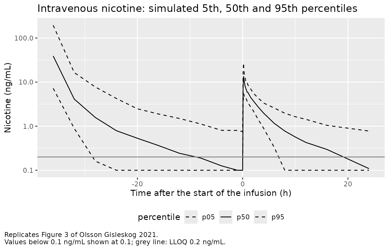
Replicating Figure 3

Figure 3 of the paper is a VPC of the intravenous data, including the washout period during which residual nicotine from smoking decays. The simulation below reproduces the study design: a virtual 1-mg bolus with VIRTUAL_DOSE = 1 at the start of the 36-h washout, then 0.028 mg/kg infused over 10 min.

times_iv <- c(seq(-36, -4, by = 4), -1, -0.5, seq(0, 1, by = 1 / 12), 1.5, 2, 3, 4, 6, 8, 10, 12, 16, 24)
ev_iv <- bind_rows(lapply(seq_len(n_arm), function(i) {
  wt <- draw_wt(1)
  d <- 0.028 * wt
  bind_rows(
    tibble(time = -36, evid = 1L, cmt = "central", amt = 1, rate = NA_real_, VIRTUAL_DOSE = 1),
    tibble(time = 0, evid = 1L, cmt = "central", amt = d, rate = d * 6, VIRTUAL_DOSE = 0),
    tibble(time = times_iv, evid = 0L, cmt = "central", amt = NA_real_, rate = NA_real_, VIRTUAL_DOSE = 0)
  ) |>
    mutate(id = i, WT = wt)
})) |>
  arrange(id, time, desc(evid))
sim_iv <- rxode2::rxSolve(mods$iv, ev_iv, returnType = "data.frame")
#> Warning: 
#> with negative times, compartments initialize at first negative observed time
#> with positive times, compartments initialize at time zero
#> use 'rxSetIni0(FALSE)' to initialize at first observed time
#> this warning is displayed once per session
sim_iv |>
  group_by(time) |>
  summarise(
    p05 = quantile(sim, 0.05), p50 = median(sim), p95 = quantile(sim, 0.95),
    .groups = "drop"
  ) |>
  pivot_longer(-time, names_to = "percentile", values_to = "Cc") |>
  mutate(Cc = pmax(Cc, 0.1)) |>
  ggplot(aes(time, Cc, linetype = percentile)) +
  geom_line() +
  geom_hline(yintercept = 0.2, colour = "grey50") +
  scale_y_log10() +
  scale_linetype_manual(values = c(p05 = "dashed", p50 = "solid", p95 = "dashed")) +
  labs(
    x = "Time after the start of the infusion (h)", y = "Nicotine (ng/mL)",
    title = "Intravenous nicotine: simulated 5th, 50th and 95th percentiles",
    caption = "Replicates Figure 3 of Olsson Gisleskog 2021.\nValues below 0.1 ng/mL shown at 0.1; grey line: LLOQ 0.2 ng/mL."
  )

# Approximate values read from the raster Figure 3 (observed percentiles and
# the proportion of observations below the limit of quantification).
fig3 <- tibble(
  time = c(-24, 1 / 6, 6, 12, 24),
  `Figure 3 median (ng/mL)` = c("1.4", "12", "1.5", "0.6", "< LLOQ"),
  `Figure 3 BQL (%)` = c("0", "0", "0", "30", "70")
)
iv_tab <- sim_iv |>
  mutate(time = round(time, 4)) |>
  filter(time %in% round(fig3$time, 4)) |>
  group_by(time) |>
  summarise(
    `Simulated 5th` = quantile(sim, 0.05), `Simulated median` = median(sim),
    `Simulated 95th` = quantile(sim, 0.95), `Simulated BQL (%)` = 100 * mean(sim < 0.2),
    .groups = "drop"
  ) |>
  inner_join(fig3 |> mutate(time = round(time, 4)), by = "time")
stopifnot(nrow(iv_tab) == nrow(fig3))
iv_tab |>
  rename(`Time (h)` = time) |>
  knitr::kable(digits = 2, caption = "Simulated IV percentiles (with residual error) vs Figure 3.")

Simulated IV percentiles (with residual error) vs Figure 3.

Time (h)	Simulated 5th	Simulated median	Simulated 95th	Simulated BQL (%)	Figure 3 median (ng/mL)	Figure 3 BQL (%)
-24.00	-0.04	0.79	4.26	15.0	1.4	0
0.17	5.44	13.42	27.05	0.0	12	0
6.00	0.33	1.16	2.59	3.0	1.5	0
12.00	-0.06	0.43	1.43	24.5	0.6	30
24.00	-0.31	0.11	0.78	57.0	< LLOQ	70

The simulated medians fall inside the model-predicted median bands drawn in Figure 3 (about 0.35-1.5 ng/mL at -24 h, 0.45-0.65 ng/mL at 12 h) and sit slightly below the observed medians, and roughly half to two-thirds of the simulated 24-h values are below the 0.2 ng/mL limit of quantification, as in the figure’s lower panel. Figure 3 itself shows the model somewhat overpredicting the spread of the data, which the paper notes (Sect. 3.2).

Oral model

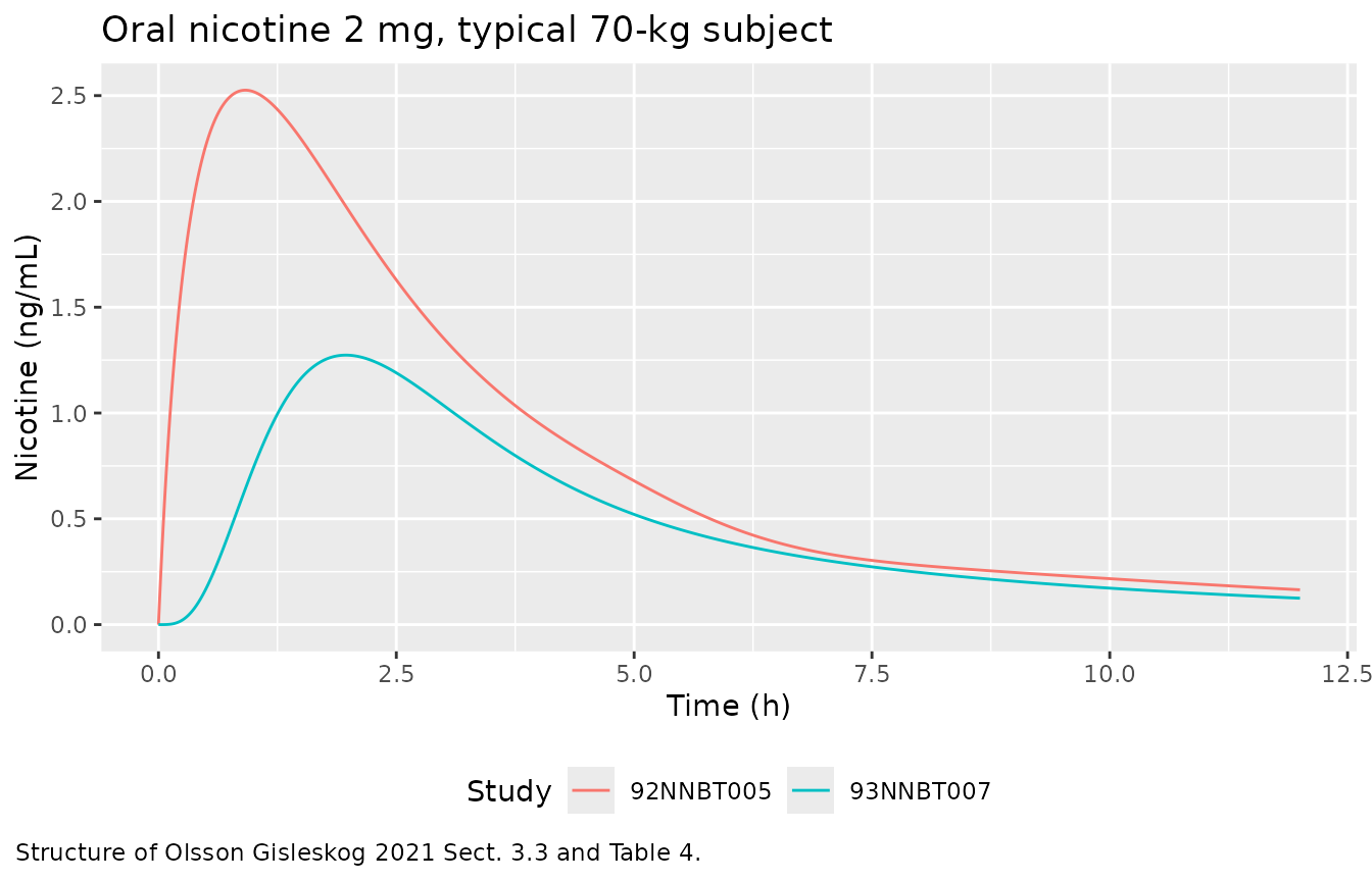
In study 92NNBT005 (microtablets chewed, repeated doses) absorption is first-order directly into central with F = 39.5%; in 93NNBT007 (tablets swallowed whole, single dose) the drug passes through three transit compartments and F is 22.3%. The typical single-dose profiles after 2 mg follow.

oral_typ <- bind_rows(lapply(0:1, function(st) {
  s <- solve_typical(
    mods$oral,
    tibble(time = 0, cmt = "depot", amt = 2, rate = NA_real_),
    list(WT = 70, STUDY_93NNBT007 = st)
  )
  tibble(time = s$time, Cc = s$Cc, study = if (st == 1) "93NNBT007" else "92NNBT005")
}))
#> ℹ omega/sigma items treated as zero: 'etalvp', 'etalvp2', 'etalvc', 'etalcl_time_dur', 'etalfcentral', 'etalktr', 'etalfdepot', 'etalcl'
#> ℹ omega/sigma items treated as zero: 'etalvp', 'etalvp2', 'etalvc', 'etalcl_time_dur', 'etalfcentral', 'etalktr', 'etalfdepot', 'etalcl'
oral_typ |>
  filter(time <= 12) |>
  ggplot(aes(time, Cc, colour = study)) +
  geom_line() +
  labs(
    x = "Time (h)", y = "Nicotine (ng/mL)", colour = "Study",
    title = "Oral nicotine 2 mg, typical 70-kg subject",
    caption = "Structure of Olsson Gisleskog 2021 Sect. 3.3 and Table 4."
  )

# Study 93NNBT007 has no time effect; for 92NNBT005 the transient clearance
# increase is switched off so that CL is constant and the identity applies.
oral_off <- rxode2::ini(mods$oral, lcl_time_max = -50)
#> ℹ change initial estimate of `lcl_time_max` to `-50`
for (st in 0:1) {
  s <- solve_typical(
    oral_off,
    tibble(time = 0, cmt = "depot", amt = 2, rate = NA_real_),
    list(WT = 70, STUDY_93NNBT007 = st)
  )
  f_oral <- exp(th(mods$oral, if (st == 1) "lfdepot_93nnbt007" else "lfdepot_92nnbt005"))
  mass_balance[[paste0("oral_", if (st == 1) "93NNBT007" else "92NNBT005")]] <- mb_error(s, 2 * f_oral)
}
#> ℹ omega/sigma items treated as zero: 'etalvp', 'etalvp2', 'etalvc', 'etalcl_time_dur', 'etalfcentral', 'etalktr', 'etalfdepot', 'etalcl'
#> ℹ omega/sigma items treated as zero: 'etalvp', 'etalvp2', 'etalvc', 'etalcl_time_dur', 'etalfcentral', 'etalktr', 'etalfdepot', 'etalcl'

Replicating Figure 7: time-dependent clearance and bioavailability

Repeated oral and buccal dosing gave lower-than-expected accumulation, which the paper describes with a transient increase in clearance (oral, mouth spray, lozenge, inhaler) or a decrease in oral bioavailability (chewing gum) following Eq. 2, where T is the time since the first dose of the treatment period. The typical time courses:

eq2 <- function(t, start, dur, pow) {
  ifelse(t > 0, 1 / (1 + (start / t)^pow) - 1 / (1 + ((start + dur) / t)^pow), 0)
}
tt <- seq(0, 24, by = 0.05)
typ_eff <- function(k) {
  m <- mods[[k]]
  if (k == "gum") {
    emax <- -plogis(th(m, "logitfdepot_oral_time_max"))
    start <- exp(th(m, "lfdepot_oral_t50"))
    dur <- exp(th(m, "lfdepot_oral_time_dur"))
    pow <- th(m, "fdepot_oral_time_hill")
  } else {
    emax <- exp(th(m, "lcl_time_max"))
    start <- exp(th(m, "lcl_t50"))
    dur <- exp(th(m, "lcl_time_dur"))
    pow <- exp(th(m, "lcl_time_hill"))
  }
  tibble(time = tt, change = 100 * emax * eq2(tt, start, dur, pow), model = k)
}
fig7 <- bind_rows(lapply(c("oral", "mouthspray", "lozenge", "inhaler", "gum"), typ_eff))
ggplot(fig7, aes(time, change, colour = model)) +
  geom_line() +
  labs(
    x = "Time since the first dose (h)", y = "Change (%)", colour = NULL,
    title = "Typical change in CL (oral, spray, lozenge, inhaler) or oral F (gum)",
    caption = "Replicates the typical-value lines of Figure 7 of Olsson Gisleskog 2021."
  )

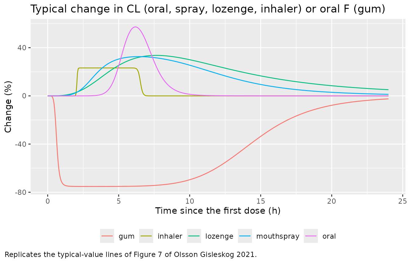
fig7_max <- fig7 |>
  group_by(model) |>
  summarise(change = change[which.max(abs(change))], .groups = "drop")
stopifnot(nrow(fig7_max) == 5)
fig7_max |>
  rename(Model = model, `Largest typical change (%)` = change) |>
  knitr::kable(digits = 1)

Model	Largest typical change (%)
gum	-75.2
inhaler	23.2
lozenge	33.6
mouthspray	32.6
oral	57.2

The paper summarises the buccal clearance increases as “around 30%”; the typical maxima above are 23-34% for the mouth spray, lozenge and inhaler (the mouth-spray and lozenge Emax estimates of 36% and 54% are not reached because onset and offset overlap), with the individual curves in Figure 7 varying widely around them because the onset, duration or Emax carry IIV. The oral repeated-dose study and the gum have larger, shorter or longer-lasting changes, as in Figure 7.

Buccal models

Fraction swallowed

fsw_tab <- tibble(
  Product = c("Mouth spray 2 mg", "Mouth spray 4 mg", "Chewing gum", "Lozenge (NiQuitin) 2 mg", "Lozenge (NiQuitin) 4 mg", "Inhaler"),
  Model = c(
    100 * plogis(th(mods$mouthspray, "logitfsw")) * (c(2, 4) / 2)^th(mods$mouthspray, "e_dose_nicotine_mg_fsw"),
    100 * plogis(th(mods$gum, "logitfsw")),
    100 * plogis(th(mods$lozenge, "logitfsw") + c(th(mods$lozenge, "e_dose2mg_fsw"), 0)),
    100 * plogis(th(mods$inhaler, "logitfsw"))
  ),
  `Table 5` = c(60.6, 64.6, 54.7, 64.0, 68.8, 66.9)
)
knitr::kable(fsw_tab, digits = 1, caption = "Typical fraction of the dose swallowed (%).")

Typical fraction of the dose swallowed (%).

Product	Model	Table 5
Mouth spray 2 mg	60.6	60.6
Mouth spray 4 mg	64.6	64.6
Chewing gum	54.7	54.7
Lozenge (NiQuitin) 2 mg	64.0	64.0
Lozenge (NiQuitin) 4 mg	68.8	68.8
Inhaler	66.9	66.9

stopifnot(all(abs(fsw_tab$Model - fsw_tab$`Table 5`) < 0.051))

These are also the values quoted in the Discussion: lowest for chewing gum (55%), then mouth spray (61%), inhaler (67%) and lozenge (69%). A Nicorette lozenge adds 0.412 on the logit scale, giving 76.9% at 4 mg.

Mass balance

With the time-dependent change switched off, CL * AUC(0-inf) must equal the dose times (1 - Frsw) * F_buccal + Frsw * F_oral. For the gum only the amount released during the 0.5-h chew counts: 1 - exp(-Krel (0.5 - lag)) of the buccal share, whose release starts after the lag, and 1 - exp(-Krel 0.5) (= released/nominal) of the swallowed share.

D <- 2
f_or <- 0.395

m <- rxode2::ini(mods$mouthspray, lcl_time_max = -50)
#> ℹ change initial estimate of `lcl_time_max` to `-50`
fsw <- plogis(th(m, "logitfsw"))
s <- solve_typical(m, tibble(time = 0, cmt = c("depot_buccal", "depot_oral"), amt = D, rate = NA_real_),
  list(WT = 70, OCC = 1, DOSE_NICOTINE_MG = D, ROUTE_SUBLINGUAL = 0))
#> Warning: some etas defaulted to non-mu referenced, possible parsing error: etaiov_ktr_6, etaiov_ktr_5, etaiov_ktr_4, etaiov_ktr_3, etaiov_ktr_2, etaiov_ktr_1, etaiov_fsw_6, etaiov_fsw_5, etaiov_fsw_4, etaiov_fsw_3, etaiov_fsw_2, etaiov_fsw_1, etaiov_ka_6, etaiov_ka_5, etaiov_ka_4, etaiov_ka_3, etaiov_ka_2, etaiov_ka_1, etaiov_fcentral_6, etaiov_fcentral_5, etaiov_fcentral_4, etaiov_fcentral_3, etaiov_fcentral_2, etaiov_fcentral_1
#> as a work-around try putting the mu-referenced expression on a simple line
#> ℹ omega/sigma items treated as zero: 'etalvp', 'etalvp2', 'etalvc', 'etaiov_ktr_6', 'etaiov_ktr_5', 'etaiov_ktr_4', 'etaiov_ktr_3', 'etaiov_ktr_2', 'etaiov_ktr_1', 'etaiov_fsw_6', 'etaiov_fsw_5', 'etaiov_fsw_4', 'etaiov_fsw_3', 'etaiov_fsw_2', 'etaiov_fsw_1', 'etaiov_ka_6', 'etaiov_ka_5', 'etaiov_ka_4', 'etaiov_ka_3', 'etaiov_ka_2', 'etaiov_ka_1', 'etaiov_fcentral_6', 'etaiov_fcentral_5', 'etaiov_fcentral_4', 'etaiov_fcentral_3', 'etaiov_fcentral_2', 'etaiov_fcentral_1', 'etalcl_time_dur', 'etalfcentral', 'etalfdepot_oral', 'etaltlag', 'etalcl'
mass_balance$mouthspray <- mb_error(s, D * ((1 - fsw) + fsw * f_or))

released_gum <- D * (1 - exp(-2.8 * 0.5)) # the paper's average Krel of 2.8 1/h
krel_gum <- -log(1 - released_gum / D) / 0.5
lag_gum <- exp(th(mods$gum, "ltlag"))
fsw <- plogis(th(mods$gum, "logitfsw"))
s <- solve_typical(mods$gum, tibble(time = 0, cmt = c("depot", "depot_oral"), amt = D, rate = NA_real_),
  list(WT = 70, OCC = 1, DOSE_NICOTINE_MG = D, DOSE_NICOTINE_RELEASED_MG = released_gum, FORM_NICOTINE_FRESHMINT = 0))
#> Warning: some etas defaulted to non-mu referenced, possible parsing error: etaiov_fcentral_5, etaiov_fcentral_4, etaiov_fcentral_3, etaiov_fcentral_2, etaiov_fcentral_1, etaiov_fsw_5, etaiov_fsw_4, etaiov_fsw_3, etaiov_fsw_2, etaiov_fsw_1
#> as a work-around try putting the mu-referenced expression on a simple line
#> ℹ omega/sigma items treated as zero: 'etalvp', 'etalvp2', 'etalvc', 'etaiov_fcentral_5', 'etaiov_fcentral_4', 'etaiov_fcentral_3', 'etaiov_fcentral_2', 'etaiov_fcentral_1', 'etaiov_fsw_5', 'etaiov_fsw_4', 'etaiov_fsw_3', 'etaiov_fsw_2', 'etaiov_fsw_1', 'etalfcentral', 'etalfdepot_oral_time_dur', 'etalfdepot_oral_t50', 'etalogitfdepot_oral_time_max', 'etalfdepot_oral', 'etaltlag', 'etalcl'
mass_balance$gum <- mb_error(s, D * ((1 - fsw) * (1 - exp(-krel_gum * (0.5 - lag_gum))) + fsw * f_or * (1 - exp(-krel_gum * 0.5))))

m <- rxode2::ini(mods$lozenge, lcl_time_max = -50)
#> ℹ change initial estimate of `lcl_time_max` to `-50`
fsw <- plogis(th(m, "logitfsw") + th(m, "e_form_nicotine_nicorette_lozenge_fsw") + th(m, "e_dose2mg_fsw"))
s <- solve_typical(m, tibble(time = 0, cmt = c("depot", "depot_oral"), amt = D, rate = NA_real_),
  list(WT = 70, OCC = 1, DOSE_NICOTINE_MG = D, FORM_NICOTINE_NICORETTE_LOZENGE = 1))
#> Warning: some etas defaulted to non-mu referenced, possible parsing error: etaiov_ktr_5, etaiov_ktr_4, etaiov_ktr_3, etaiov_ktr_2, etaiov_ktr_1, etaiov_krel_5, etaiov_krel_4, etaiov_krel_3, etaiov_krel_2, etaiov_krel_1, etaiov_fsw_5, etaiov_fsw_4, etaiov_fsw_3, etaiov_fsw_2, etaiov_fsw_1, etaiov_fcentral_5, etaiov_fcentral_4, etaiov_fcentral_3, etaiov_fcentral_2, etaiov_fcentral_1
#> as a work-around try putting the mu-referenced expression on a simple line
#> ℹ omega/sigma items treated as zero: 'etalvp', 'etalvp2', 'etalvc', 'etaiov_ktr_5', 'etaiov_ktr_4', 'etaiov_ktr_3', 'etaiov_ktr_2', 'etaiov_ktr_1', 'etaiov_krel_5', 'etaiov_krel_4', 'etaiov_krel_3', 'etaiov_krel_2', 'etaiov_krel_1', 'etaiov_fsw_5', 'etaiov_fsw_4', 'etaiov_fsw_3', 'etaiov_fsw_2', 'etaiov_fsw_1', 'etaiov_fcentral_5', 'etaiov_fcentral_4', 'etaiov_fcentral_3', 'etaiov_fcentral_2', 'etaiov_fcentral_1', 'etalcl_time_dur', 'etalcl_t50', 'etalfdepot_buccal', 'etalfcentral', 'etalfdepot_oral', 'etalka', 'etaltlag', 'etalcl'
mass_balance$lozenge <- mb_error(s, D * ((1 - fsw) + fsw * f_or))

m <- rxode2::ini(mods$inhaler, lcl_time_max = -50)
#> ℹ change initial estimate of `lcl_time_max` to `-50`
fsw <- plogis(th(m, "logitfsw"))
for (st in 0:1) {
  s <- solve_typical(m, tibble(time = 0, cmt = c("depot_buccal", "depot_oral"), amt = D, rate = D * 3),
    list(WT = 70, OCC = 1, STUDY_97NNIN024 = st))
  f_study <- 1 + th(m, "e_study_97nnin024_f") * st
  mass_balance[[paste0("inhaler_study97NNIN024_", st)]] <- mb_error(s, D * f_study * ((1 - fsw) + fsw * f_or))
}
#> Warning: some etas defaulted to non-mu referenced, possible parsing error: etaiov_ktr_2, etaiov_ktr_1, etaiov_fsw_2, etaiov_fsw_1, etaiov_fcentral_2, etaiov_fcentral_1
#> as a work-around try putting the mu-referenced expression on a simple line
#> ℹ omega/sigma items treated as zero: 'etalvp', 'etalvp2', 'etalvc', 'etaiov_ktr_2', 'etaiov_ktr_1', 'etaiov_fsw_2', 'etaiov_fsw_1', 'etaiov_fcentral_2', 'etaiov_fcentral_1', 'etalcl_time_max', 'etalcl_time_dur', 'etalfcentral', 'etalfdepot_oral', 'etalfdepot_buccal', 'etalcl'
#> Warning: some etas defaulted to non-mu referenced, possible parsing error: etaiov_ktr_2, etaiov_ktr_1, etaiov_fsw_2, etaiov_fsw_1, etaiov_fcentral_2, etaiov_fcentral_1
#> as a work-around try putting the mu-referenced expression on a simple line
#> ℹ omega/sigma items treated as zero: 'etalvp', 'etalvp2', 'etalvc', 'etaiov_ktr_2', 'etaiov_ktr_1', 'etaiov_fsw_2', 'etaiov_fsw_1', 'etaiov_fcentral_2', 'etaiov_fcentral_1', 'etalcl_time_max', 'etalcl_time_dur', 'etalfcentral', 'etalfdepot_oral', 'etalfdepot_buccal', 'etalcl'

Replicating Figure 11

Figure 11 compares simulated single doses of a 2-mg mouth spray, 2-mg Nicorette classic gum, 2-mg Nicorette lozenge and the inhaler (means and 90% prediction intervals). The gum is simulated with the released amount that gives the paper’s average release rate of 2.8 1/h (75% of the nominal dose), and the inhaler with 2 mg released over a 20-min session, the average reported in Sect. 3.4.

t_buc <- c(seq(0, 1, by = 1 / 12), seq(1.25, 3, by = 0.25), 3.5, 4:12)
ev_buc <- bind_rows(
  make_arm(tibble(time = 0, cmt = c("depot_buccal", "depot_oral"), amt = 2, rate = NA_real_), t_buc,
    list(OCC = 1, DOSE_NICOTINE_MG = 2, ROUTE_SUBLINGUAL = 0), "Mouth spray 2 mg", 0L),
  make_arm(tibble(time = 0, cmt = c("depot", "depot_oral"), amt = 2, rate = NA_real_), t_buc,
    list(OCC = 1, DOSE_NICOTINE_MG = 2, DOSE_NICOTINE_RELEASED_MG = released_gum, FORM_NICOTINE_FRESHMINT = 0),
    "Nicorette gum classic 2 mg", 1000L),
  make_arm(tibble(time = 0, cmt = c("depot", "depot_oral"), amt = 2, rate = NA_real_), t_buc,
    list(OCC = 1, DOSE_NICOTINE_MG = 2, FORM_NICOTINE_NICORETTE_LOZENGE = 1), "Nicorette lozenge 2 mg", 2000L),
  make_arm(tibble(time = 0, cmt = c("depot_buccal", "depot_oral"), amt = 2, rate = 2 * 3), t_buc,
    list(OCC = 1, STUDY_97NNIN024 = 0), "Nicorette inhaler (2 mg released)", 3000L)
)
stopifnot(!anyDuplicated(unique(ev_buc[, c("id", "time", "evid", "cmt")])))
buc_model <- c(
  "Mouth spray 2 mg" = "mouthspray", "Nicorette gum classic 2 mg" = "gum",
  "Nicorette lozenge 2 mg" = "lozenge", "Nicorette inhaler (2 mg released)" = "inhaler"
)
sim_buc <- bind_rows(lapply(names(buc_model), function(trt) {
  ev <- ev_buc |>
    filter(treatment == trt) |>
    select(where(~ !all(is.na(.x))))
  rxode2::rxSolve(mods[[buc_model[[trt]]]], ev, keep = "treatment", returnType = "data.frame")
}))
buc_sum <- sim_buc |>
  group_by(treatment, time) |>
  summarise(mean = mean(Cc), p05 = quantile(Cc, 0.05), p95 = quantile(Cc, 0.95), .groups = "drop")
ggplot(buc_sum, aes(time, mean, colour = treatment, fill = treatment)) +
  geom_ribbon(aes(ymin = p05, ymax = p95), alpha = 0.15, colour = NA) +
  geom_line() +
  labs(
    x = "Time (h)", y = "Nicotine (ng/mL)", colour = NULL, fill = NULL,
    title = "Single doses of four buccal products",
    caption = "Replicates Figure 11 of Olsson Gisleskog 2021 (means and 90% prediction intervals)."
  ) +
  guides(colour = guide_legend(ncol = 2), fill = guide_legend(ncol = 2))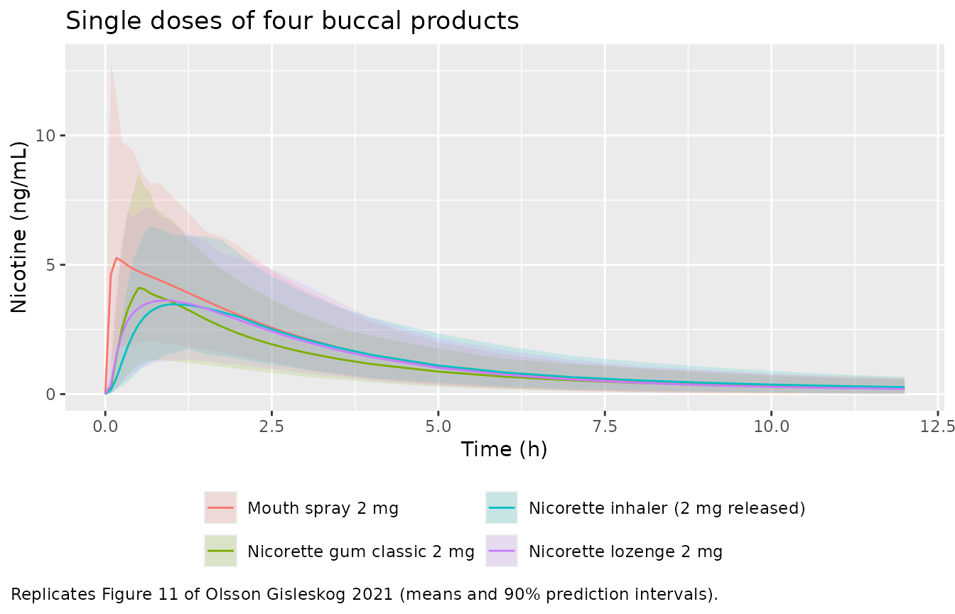

# Peaks of the MEAN curves read by eye from the raster Figure 11 (about
# +/- 0.2 ng/mL, +/- 5 min). The published inhaler curve is labelled
# '15-mg inhaler' without the released amount, so it is shown but not gated.
fig11 <- tibble(
  treatment = names(buc_model),
  `Figure 11 peak (ng/mL)` = c(4.9, 3.5, 3.6, 4.5),
  `Figure 11 time of peak (h)` = c(0.17, 0.5, 1.0, 1.0),
  gated = c(TRUE, TRUE, TRUE, FALSE)
)
fig11_cmp <- buc_sum |>
  group_by(treatment) |>
  summarise(`Simulated peak (ng/mL)` = max(mean), `Simulated time of peak (h)` = time[which.max(mean)], .groups = "drop") |>
  inner_join(fig11, by = "treatment") |>
  mutate(`Difference (%)` = 100 * (`Simulated peak (ng/mL)` / `Figure 11 peak (ng/mL)` - 1))
stopifnot(nrow(fig11_cmp) == 4)
fig11_cmp |>
  select(-gated) |>
  knitr::kable(digits = 2, caption = "Peak of the simulated mean curve vs Figure 11.")

Peak of the simulated mean curve vs Figure 11.

treatment	Simulated peak (ng/mL)	Simulated time of peak (h)	Figure 11 peak (ng/mL)	Figure 11 time of peak (h)	Difference (%)
Mouth spray 2 mg	5.27	0.17	4.9	0.17	7.49
Nicorette gum classic 2 mg	4.11	0.50	3.5	0.50	17.33
Nicorette inhaler (2 mg released)	3.48	1.00	4.5	1.00	-22.73
Nicorette lozenge 2 mg	3.63	0.92	3.6	1.00	0.69

# Over 8 seeds (identical at 1 and 4 solver threads) the differences were
# -3.5 to +4.2% (spray), +7.8 to +18.8% (gum; systematically high, see the
# text) and -7.5 to +2.7% (lozenge), so 30% leaves at least 11 points of
# headroom. A transcription error in a rate constant, a fraction swallowed or
# a unit moves the peak by far more.
stopifnot(all(abs(fig11_cmp$`Difference (%)`[fig11_cmp$gated]) < 30))

The mouth spray, gum and lozenge reproduce Figure 11 in both height and timing of the mean peak. The gum peak is about 10% higher than the figure in every cohort drawn while developing this article, which is consistent with the released amount assumed here (the paper does not state the one it simulated). The simulated inhaler peak is lower than the published one (see Assumptions and deviations).

Transdermal model

Mass balance

The first-order pathway is scaled so that the whole fraction Fr1 of the bioavailable dose leaves the patch within its release window of Frdur1 x 16 h. For the Invisipatch the window is timed from application but the first-order release only starts after the 0.53-h lag, so slightly less than Fr1 is released; the zero-order pathway delivers FTOT (1 - Fr1) between 4.06 h and patch removal.

m <- rxode2::ini(mods$transdermal, lcl_time_max = -50)
#> ℹ change initial estimate of `lcl_time_max` to `-50`
for (inv in 0:1) {
  sfx <- if (inv == 1) "invisipatch" else "nicorette"
  s <- solve_typical(m, tibble(time = 0, cmt = c("depot_td", "transit1"), amt = 25, rate = c(NA_real_, -2)),
    list(WT = 70, OCC = 1, FORM_NICOTINE_INVISIPATCH = inv, T_PATCH_WEAR = 16))
  ftot <- exp(th(m, "lfdepot"))
  ffo <- plogis(th(m, paste0("logitffo_", sfx)))
  dd <- 16 * plogis(th(m, paste0("logitfrdur_", sfx)))
  kr <- exp(th(m, "lkrel"))
  lag1 <- if (inv == 1) exp(th(m, "ltlag_invisipatch")) else 0
  expected <- 25 * ftot * (ffo * (1 - exp(-kr * (dd - lag1))) / (1 - exp(-kr * dd)) + (1 - ffo))
  mass_balance[[paste0("patch_", sfx)]] <- mb_error(s, expected)
}
#> Warning: some etas defaulted to non-mu referenced, possible parsing error: etaiov_fdepot_6, etaiov_fdepot_5, etaiov_fdepot_4, etaiov_fdepot_3, etaiov_fdepot_2, etaiov_fdepot_1, etaiov_fcentral_6, etaiov_fcentral_5, etaiov_fcentral_4, etaiov_fcentral_3, etaiov_fcentral_2, etaiov_fcentral_1
#> as a work-around try putting the mu-referenced expression on a simple line
#> ℹ omega/sigma items treated as zero: 'etalvp', 'etalvp2', 'etalvc', 'etaiov_fdepot_6', 'etaiov_fdepot_5', 'etaiov_fdepot_4', 'etaiov_fdepot_3', 'etaiov_fdepot_2', 'etaiov_fdepot_1', 'etaiov_fcentral_6', 'etaiov_fcentral_5', 'etaiov_fcentral_4', 'etaiov_fcentral_3', 'etaiov_fcentral_2', 'etaiov_fcentral_1', 'etalfcentral', 'etalogitffo', 'etalogitfrdur', 'etalktr', 'etalkrel', 'etalcl'
#> Warning: some etas defaulted to non-mu referenced, possible parsing error: etaiov_fdepot_6, etaiov_fdepot_5, etaiov_fdepot_4, etaiov_fdepot_3, etaiov_fdepot_2, etaiov_fdepot_1, etaiov_fcentral_6, etaiov_fcentral_5, etaiov_fcentral_4, etaiov_fcentral_3, etaiov_fcentral_2, etaiov_fcentral_1
#> as a work-around try putting the mu-referenced expression on a simple line
#> ℹ omega/sigma items treated as zero: 'etalvp', 'etalvp2', 'etalvc', 'etaiov_fdepot_6', 'etaiov_fdepot_5', 'etaiov_fdepot_4', 'etaiov_fdepot_3', 'etaiov_fdepot_2', 'etaiov_fdepot_1', 'etaiov_fcentral_6', 'etaiov_fcentral_5', 'etaiov_fcentral_4', 'etaiov_fcentral_3', 'etaiov_fcentral_2', 'etaiov_fcentral_1', 'etalfcentral', 'etalogitffo', 'etalogitfrdur', 'etalktr', 'etalkrel', 'etalcl'

Replicating Figure 12

t_td <- c(seq(0, 2, by = 0.5), 3:24)
ev_td <- bind_rows(
  make_arm(tibble(time = 0, cmt = c("depot_td", "transit1"), amt = 25, rate = c(NA_real_, -2)), t_td,
    list(OCC = 1, FORM_NICOTINE_INVISIPATCH = 0, T_PATCH_WEAR = 16), "Nicorette 25 mg/16 h", 0L),
  make_arm(tibble(time = 0, cmt = c("depot_td", "transit1"), amt = 25, rate = c(NA_real_, -2)), t_td,
    list(OCC = 1, FORM_NICOTINE_INVISIPATCH = 1, T_PATCH_WEAR = 16), "Invisipatch 25 mg/16 h", 1000L)
)
stopifnot(!anyDuplicated(unique(ev_td[, c("id", "time", "evid", "cmt")])))
sim_td <- rxode2::rxSolve(mods$transdermal, ev_td, keep = "treatment", returnType = "data.frame")
td_sum <- sim_td |>
  group_by(treatment, time) |>
  summarise(mean = mean(Cc), p05 = quantile(Cc, 0.05), p95 = quantile(Cc, 0.95), .groups = "drop")
ggplot(td_sum, aes(time, mean, colour = treatment, fill = treatment)) +
  geom_ribbon(aes(ymin = p05, ymax = p95), alpha = 0.15, colour = NA) +
  geom_line() +
  scale_x_continuous(breaks = seq(0, 24, 4)) +
  labs(
    x = "Time (h)", y = "Nicotine (ng/mL)", colour = NULL, fill = NULL,
    title = "Single 25-mg/16-h patch applications",
    caption = "Replicates Figure 12 of Olsson Gisleskog 2021 (means and 90% prediction intervals)."
  )

# Mean curves read by eye from the raster Figure 12 (about +/- 0.5 ng/mL).
fig12 <- tribble(
  ~treatment, ~time, ~figure12,
  "Nicorette 25 mg/16 h", 4, 17.0,
  "Nicorette 25 mg/16 h", 8, 16.2,
  "Nicorette 25 mg/16 h", 12, 13.0,
  "Nicorette 25 mg/16 h", 16, 11.7,
  "Nicorette 25 mg/16 h", 24, 2.6,
  "Invisipatch 25 mg/16 h", 4, 13.6,
  "Invisipatch 25 mg/16 h", 8, 15.8,
  "Invisipatch 25 mg/16 h", 12, 14.2,
  "Invisipatch 25 mg/16 h", 16, 11.7,
  "Invisipatch 25 mg/16 h", 24, 2.6
)
fig12_cmp <- fig12 |>
  inner_join(td_sum |> select(treatment, time, simulated = mean), by = c("treatment", "time")) |>
  mutate(`Difference (%)` = 100 * (simulated / figure12 - 1))
stopifnot(nrow(fig12_cmp) == nrow(fig12))
fig12_cmp |>
  rename(`Time (h)` = time, `Figure 12 mean (ng/mL)` = figure12, `Simulated mean (ng/mL)` = simulated) |>
  knitr::kable(digits = 1, caption = "Simulated mean concentration vs Figure 12.")

Simulated mean concentration vs Figure 12.

treatment	Time (h)	Figure 12 mean (ng/mL)	Simulated mean (ng/mL)	Difference (%)
Nicorette 25 mg/16 h	4	17.0	10.3	-39.3
Nicorette 25 mg/16 h	8	16.2	14.5	-10.8
Nicorette 25 mg/16 h	12	13.0	13.8	5.8
Nicorette 25 mg/16 h	16	11.7	13.3	13.5
Nicorette 25 mg/16 h	24	2.6	3.2	23.4
Invisipatch 25 mg/16 h	4	13.6	12.7	-6.7
Invisipatch 25 mg/16 h	8	15.8	16.4	3.9
Invisipatch 25 mg/16 h	12	14.2	15.0	5.3
Invisipatch 25 mg/16 h	16	11.7	12.6	7.3
Invisipatch 25 mg/16 h	24	2.6	3.2	24.0

# Invisipatch during wear (4-16 h): gated. Over 8 seeds the differences were
# -10.9 to +8.5%, so 25% leaves 14 points of headroom. The 24-h point (8 h
# after removal) and the Nicorette patch are discussed below and not gated.
inv_wear <- fig12_cmp |> filter(treatment == "Invisipatch 25 mg/16 h", time <= 16)
stopifnot(nrow(inv_wear) == 4, all(abs(inv_wear$`Difference (%)`) < 25))

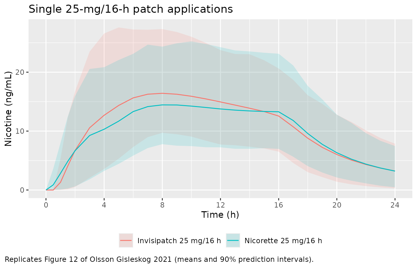
The Invisipatch reproduces Figure 12 during the application period. The Nicorette patch does not: the model rises more slowly (-39% against the published mean at 4 h) and stays higher towards removal (+14% at 16 h). The simulated Nicorette profile does, however, agree with the simulated median of the paper’s own VPC for the 25-mg Nicorette patch (Figure 10, STRT 3: about 12-14 ng/mL from 8 to 12 h, peak observed around 10 h, Sect. 3.5), and the parameters are those printed in Table 6 and in the final NONMEM output. The difference is therefore attributed to Figure 12 rather than to the model; see Assumptions and deviations.

Replicating Figure 10 (STRT 7 and 8): three daily Invisipatch applications

t_rep <- c(seq(0, 72, by = 1))
ev_rep <- bind_rows(lapply(c(16, 24), function(wear) {
  make_arm(
    tibble(time = rep(c(0, 24, 48), each = 2), cmt = rep(c("depot_td", "transit1"), 3), amt = 25, rate = rep(c(NA_real_, -2), 3)),
    t_rep, list(OCC = 1, FORM_NICOTINE_INVISIPATCH = 1, T_PATCH_WEAR = wear),
    paste0("Invisipatch 25 mg worn ", wear, " h"), if (wear == 16) 0L else 1000L
  )
}))
sim_rep <- rxode2::rxSolve(mods$transdermal, ev_rep, keep = "treatment", returnType = "data.frame")
sim_rep |>
  group_by(treatment, time) |>
  summarise(p05 = quantile(Cc, 0.05), p50 = median(Cc), p95 = quantile(Cc, 0.95), .groups = "drop") |>
  ggplot(aes(time, p50)) +
  geom_ribbon(aes(ymin = p05, ymax = p95), alpha = 0.2) +
  geom_line() +
  facet_wrap(~treatment) +
  scale_x_continuous(breaks = seq(0, 72, 12)) +
  labs(
    x = "Time (h)", y = "Nicotine (ng/mL)",
    title = "Three daily 25-mg Invisipatch applications",
    caption = "Replicates the simulated median and 5th-95th percentiles of Figure 10\n(STRT 7 and 8) of Olsson Gisleskog 2021."
  )

rep_tab <- sim_rep |>
  group_by(treatment, time) |>
  summarise(median = median(Cc), .groups = "drop") |>
  group_by(treatment) |>
  summarise(
    `Day 1 peak (ng/mL)` = max(median[time <= 24]),
    `Trough before day 2 (ng/mL)` = median[time == 24],
    `Day 3 peak (ng/mL)` = max(median[time >= 48 & time <= 72]),
    .groups = "drop"
  )
stopifnot(nrow(rep_tab) == 2)
knitr::kable(rep_tab, digits = 1, caption = "Median profile features for three daily 25-mg Invisipatch applications.")

Median profile features for three daily 25-mg Invisipatch applications.

treatment	Day 1 peak (ng/mL)	Trough before day 2 (ng/mL)	Day 3 peak (ng/mL)
Invisipatch 25 mg worn 16 h	15.3	2.4	17.7
Invisipatch 25 mg worn 24 h	14.5	5.1	17.1

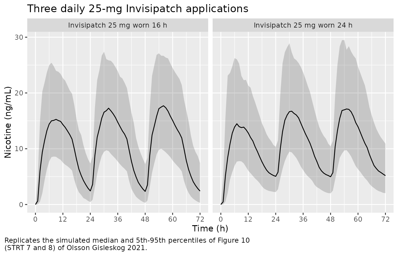
Sect. 3.5 reports that keeping the patch on for 24 h raised the trough without a large difference in peak exposure; the table shows the same pattern in the simulation.

Mass-balance summary

mb <- tibble(Check = names(mass_balance), `Relative error` = unlist(mass_balance))
knitr::kable(mb, digits = 8, caption = "CL * AUC(0-inf) against the expected bioavailable amount (typical values, tight solver tolerances).")

CL * AUC(0-inf) against the expected bioavailable amount (typical values, tight solver tolerances).

Check	Relative error
iv	-5.91e-06
oral_92NNBT005	2.02e-06
oral_93NNBT007	2.48e-06
mouthspray	9.25e-06
gum	4.22e-06
lozenge	4.17e-06
inhaler_study97NNIN024_0	3.73e-06
inhaler_study97NNIN024_1	3.75e-06
patch_nicorette	5.00e-08
patch_invisipatch	1.07e-06

# Realised errors are below 1e-5 (trapezoid rule on the dense grid); a
# mis-set bioavailability, dose split, lag or release window moves them by
# at least a few percent.
stopifnot(length(mass_balance) == 10, all(abs(mb$`Relative error`) < 1e-4))

PKNCA

The paper reports no non-compartmental results. For reference, PKNCA summaries of the simulated single-dose cohorts of Figures 11 and 12 follow.

nca_one <- function(sim, end) {
  conc <- sim |>
    filter(!is.na(Cc)) |>
    mutate(Cc = pmax(Cc, 0)) |>
    select(id, time, Cc, treatment)
  conc <- bind_rows(conc, distinct(conc, id, treatment) |> mutate(time = 0, Cc = 0)) |>
    distinct(id, treatment, time, .keep_all = TRUE) |>
    arrange(treatment, id, time)
  dose <- distinct(conc, id, treatment) |> mutate(time = 0, amt = 1)
  conc_obj <- PKNCA::PKNCAconc(conc, Cc ~ time | treatment + id, concu = "ng/mL", timeu = "h")
  dose_obj <- PKNCA::PKNCAdose(dose, amt ~ time | treatment + id, doseu = "mg")
  intervals <- data.frame(start = 0, end = end, cmax = TRUE, tmax = TRUE, auclast = TRUE)
  PKNCA::pk.nca(PKNCA::PKNCAdata(conc_obj, dose_obj, intervals = intervals))
}
nca_buc <- nca_one(sim_buc, 12)
nca_td <- nca_one(sim_td, 24)
nca_tab <- bind_rows(as.data.frame(nca_buc), as.data.frame(nca_td)) |>
  group_by(treatment, PPTESTCD) |>
  summarise(median = median(PPORRES), .groups = "drop") |>
  pivot_wider(names_from = PPTESTCD, values_from = median)
stopifnot(nrow(nca_tab) == 6)
nca_tab |>
  select(treatment, cmax, tmax, auclast) |>
  rename(
    Treatment = treatment, `Cmax (ng/mL)` = cmax, `Tmax (h)` = tmax,
    `AUC0-last (ng*h/mL; 0-12 h buccal, 0-24 h patch)` = auclast
  ) |>
  knitr::kable(digits = 2, caption = "Median simulated single-dose NCA (virtual subjects without residual pre-study nicotine).")

Median simulated single-dose NCA (virtual subjects without residual pre-study nicotine).

Treatment	Cmax (ng/mL)	Tmax (h)	AUC0-last (ng*h/mL; 0-12 h buccal, 0-24 h patch)
Invisipatch 25 mg/16 h	17.05	8.00	253.19
Mouth spray 2 mg	5.27	0.25	16.59
Nicorette 25 mg/16 h	15.54	9.00	230.88
Nicorette gum classic 2 mg	4.06	0.58	12.35
Nicorette inhaler (2 mg released)	3.43	1.12	13.70
Nicorette lozenge 2 mg	3.91	0.92	13.33

Assumptions and deviations

• Source of the values. Parameter values were taken from the paper’s Tables 3-6 and cross-checked against the final NONMEM control streams and output listings in the electronic supplementary material. Where the paper prints three significant figures and the extravascular control streams carry the intravenous estimates to more (for example CL 67.4 vs 67.4136 L/h), the longer value is used; the two agree to the printed precision.
• Lozenge duration and pow (Table 5 misprint). Table 5 prints 20.2 h and 9.88 as the lozenge ‘Duration’ and ‘pow’. The final NONMEM output gives 7.18 h (standard error 1.45) and 3.18 (standard error 0.314), whose relative standard errors are 20.2% and 9.87%: the table printed each RSE in the estimate column. The model uses 7.18 h and 3.18. Every other lozenge value in Table 5 matches the output.
• Gum ka footnotes. Table 5 footnote f gives Ka = Ka2mg + (1/NDOSE)^0.507 and footnote d refers to ‘3 mg of Nicorette classic’. The control stream computes KA = THETA * (NDOSE/2)^0.507 with 2 mg as the reference for both gums; the model follows the control stream.
• Time since the first dose. Eq. 2 uses the time since the first dose of the study period (dataset column TSSP). The models compute it with rxode2’s tafd() on a compartment that has no lag (the gut dose for the buccal products; the patch dose plus its lag for the patch). NONMEM evaluated TSSP only at data records, so its clearance changed in steps between records while rxode2 changes it continuously. For multi-period (crossover) simulations, simulate each period as its own subject or reset the system between periods, and set OCC to the period number: tafd() counts from the first dose ever given to the subject.
• Inhaler input. The inhaler dose records carry a fixed infusion rate (released amount over 20 min), as in the source data. With a fixed rate, bioavailability shortens the input rather than lowering its rate (NONMEM and rxode2 behave the same way), so the effective input lasts F x 20 min. Supply rate = amt * 3 rather than a modelled duration.
• Parameters fixed to zero in the source. The inhaler control stream carries an IIV on the onset time of the clearance change fixed to 0, and the lozenge control stream a NiQuitin effect on Krel fixed to 0. Both are omitted: they have no effect, and a zero variance would make the OMEGA matrix singular.
• Patch release window after a repeat application. The first-order window is timed from each application. For the Invisipatch, rxode2 measures the time from the lagged (0.53 h) arrival of the new dose, so during the first 0.53 h after a repeat application the small residue left in the first-order pool from the previous patch is not released as it would be in NONMEM. The effect on concentrations is negligible.
• Figure 12, Nicorette patch. The simulated mean for the 25-mg Nicorette patch is about 40% below Figure 12 at 4 h and 10-15% above it at 16 h, while the Invisipatch agrees. The model uses the published Table 6 values, which match the final NONMEM output, and it agrees with the paper’s own VPC for this product (Figure 10, STRT 3). No correction notice for the article was found (checked 2026-09-28). The difference is left as a documented deviation; the parameters were not adjusted.
• Figure 11, inhaler. The published curve is labelled ‘15-mg inhaler’ without the amount released or the number of sessions. Simulating the reported average of 2 mg released in one 20-min session gives a mean peak of 3.5 ng/mL against about 4.5 ng/mL in the figure. The inhaler is therefore not gated against Figure 11.
• Simulation inputs not given in the paper. Body weights are drawn from a log-normal distribution matching Table 2. The gum simulation uses a released amount of 75% of the nominal dose, which reproduces the paper’s average release rate constant of 2.8 1/h. The simulations for Figures 11 and 12 omit residual pre-study nicotine (no virtual pre-washout dose).
• Data below the limit of quantification. The intravenous model was fitted with the M3 method and the other models excluded such data. This affects estimation only and has no counterpart in the simulation models.