Amikacin (van der Veer 2025)
Source:vignettes/articles/vanderVeer_2025_amikacin.Rmd
vanderVeer_2025_amikacin.RmdModel and source
- Citation: van der Veer MAA, Smits A, de Haan TR, Franken LGW, van Kaam AH, Hodiamont CJ, Bijleveld YA, Allegaert K, Mathot RAA. Amikacin dosing in neonates: evaluation of target attainment using a simplified and complex pharmacokinetic model-derived dosing regimen in clinical practice. Antimicrob Agents Chemother. 2025;69(4):e01118-24. doi:10.1128/aac.01118-24
- Description: Two-compartment IV-infusion population PK model for amikacin in neonates (van der Veer 2025 ‘optimized’ model: the De Cock 2012 structure re-estimated on pooled Amsterdam UMC and University Hospitals Leuven NICU data). Clearance scales as a power of birth weight (reference 1685 g) times a linear function of postnatal age (1 + n * PNA / 5 days); central volume scales as a power of current weight (reference 1700 g); peripheral volume equals central volume and intercompartmental clearance is proportional to clearance (Q = 0.468 x CL). IIV on CL, and a 30% IIV on V1 set by the authors; combined additive and proportional residual error.
- Article: https://doi.org/10.1128/aac.01118-24 (open access; the model parameters are in Supplementary Data 4, Table S5)
van der Veer et al. compared amikacin target attainment in neonates treated with a simplified dosing regimen (Amsterdam UMC: 15 mg/kg every 36 h below 30 weeks’ gestation, every 24 h otherwise; paper Table 2) and with the complex De Cock 2012 model-derived regimen (University Hospitals Leuven: 15-20 mg/kg every 20-48 h by postnatal age and current weight; paper Table 1). The De Cock 2012 model under-predicted peak concentrations in the Amsterdam data, so the authors pooled both centres, re-estimated the De Cock structure on a random 75% of the neonates and added a fixed 30% IIV on the central volume. That “optimized PK model” (Supplement Table S5) is the model packaged here; the paper used it to compute each neonate’s Cmax, Cmin and AUC over the first dosing interval (Figure 1).
Population
The two cohorts are described in Table 3 of the paper. Amsterdam UMC contributed 366 neonates (768 concentrations, 2018-2024): median gestational age 28.7 weeks (24.0-42.1), postnatal age 9 days (0-31), birth weight 1100 g (440-5200), current weight 1100 g (455-5500), 59% male. University Hospitals Leuven contributed 579 neonates (1195 concentrations, 2011-2012): median gestational age 34 weeks (24-41), postnatal age 2 days (1-30), birth weight 2150 g (420-4850), current weight 2120 g (420-5040), 56% male. Ibuprofen was co-administered in 2% and 5% of the cohorts. Amikacin was infused over 20-30 minutes and concentrations were measured by immunoassay (LLOQ 0.8 mg/L).
The pooled data were split at random into a model-building dataset (75%, 710 neonates, 1412 samples) and a validation dataset. The model-building dataset is characterised in Table S5 only by its covariate medians: birth weight 1685 g, current weight 1700 g, postnatal age 5 days.
The same information is available programmatically via
readModelDb("vanderVeer_2025_amikacin")()$population.
Source trace
The per-parameter origin is recorded as an in-file comment next to
each ini() entry in
inst/modeldb/specificDrugs/vanderVeer_2025_amikacin.R.
| Equation / parameter | Value | Source location |
|---|---|---|
lcl (CLp, L/h) |
log(0.044) | Table S5, model-building dataset |
e_wt_birth_cl (m) |
1.34 | Table S5 |
e_pna_cl (n) |
0.597 | Table S5 |
lvc (Vp, L) |
log(0.794) | Table S5 |
e_wt_vc (p) |
0.903 | Table S5 |
qclratio (r) |
0.468 | Table S5 (Q = r x CL) |
etalcl |
0.0856 | Table S5, IIV on CL (variance) |
etalvc |
fixed(0.09) | Table S5 and Results: IIV on V1 fixed at 30% |
propSd |
sqrt(0.0279) = 0.167 | Table S5, proportional error (variance) |
addSd (mg/L) |
sqrt(0.378) = 0.615 | Table S5, additive error (variance) |
| CL = CLp (bBW/1685)^m (1 + n PNA/5) | n/a | Table S5 equation; medians in footnote b |
| V1 = Vp (cBW/1700)^p, V2 = V1 | n/a | Table S5 equation; medians in footnote b |
| Ibuprofen factor o = 1 (no effect) | n/a | Table S5 footnote c |
| Two-compartment model, IV infusion | n/a | Supplementary Data 1; Methods ‘Dosing and blood sampling’ |
Virtual cohorts
The individual data are not public. Two virtual cohorts of 200 neonates each approximate the Table 3 demographics of the two centres. Gestational age and postnatal age are drawn from piecewise-linear quantile functions through the reported minimum, median and maximum plus the percentage below 30 weeks and at or above 37 weeks (Table 3) and the percentage at or above 14 days of postnatal age (Table S1). Birth weight follows an approximate median birth-weight-for-gestational-age curve with 15% log-normal scatter, rescaled so that each cohort’s median equals Table 3 (NICU neonates are lighter than the curve), and current weight equals birth weight with 5% scatter (the two medians differ by less than 2% in both cohorts).
set.seed(20250311)
n_per_arm <- 200

# Piecewise-linear inverse CDF through reported quantiles.
qpw <- function(u, p, q) stats::approx(p, q, xout = u, ties = "ordered")$y

# Approximate median birth weight (kg) by gestational age (weeks).
bw_median <- function(ga) {
  stats::approx(
    c(23, 24, 28, 32, 36, 40, 43),
    c(0.55, 0.65, 1.15, 1.80, 2.75, 3.50, 3.70),
    xout = ga, rule = 2
  )$y
}

make_cohort <- function(n, ga_p, ga_q, pna_p, pna_q, bw_target, regimen, id_offset) {
  ga <- qpw(stats::runif(n), ga_p, ga_q)
  wt_birth <- bw_median(ga) * exp(stats::rnorm(n, 0, 0.15))
  # NICU cohorts are lighter than the reference curve; rescale so the cohort
  # median birth weight equals Table 3.
  wt_birth <- wt_birth * bw_target / stats::median(wt_birth)
  tibble(
    id = id_offset + seq_len(n),
    regimen = regimen,
    GA = ga,
    pna_days = qpw(stats::runif(n), pna_p, pna_q),
    WT_BIRTH = pmin(pmax(wt_birth, 0.42), 5.2),
    WT = pmin(pmax(wt_birth * exp(stats::rnorm(n, 0, 0.05)), 0.42), 5.5)
  ) |>
    mutate(PNA = pna_days / 30.4375)
}

cohort <- bind_rows(
  # Amsterdam UMC: GA 24-42.1 (median 28.7, 56.9% < 30, 12.5% >= 37);
  # PNA 0-30 days (median 9; 80 of 367 neonates >= 14 days, Table S1).
  make_cohort(
    n_per_arm,
    ga_p = c(0, 0.5, 0.569, 0.875, 1), ga_q = c(24, 28.7, 30, 37, 42.1),
    pna_p = c(0, 0.5, 0.782, 1), pna_q = c(0, 9, 14, 30),
    bw_target = 1.100, regimen = "Simplified", id_offset = 0L
  ),
  # University Hospitals Leuven: GA 24-41 (median 34, 15.7% < 30,
  # 36.6% >= 37); PNA 1-30 days (median 2; 32 of 579 >= 14 days).
  make_cohort(
    n_per_arm,
    ga_p = c(0, 0.157, 0.5, 0.634, 1), ga_q = c(24, 30, 34, 37, 41),
    pna_p = c(0, 0.5, 0.945, 1), pna_q = c(1, 2, 14, 30),
    bw_target = 2.150, regimen = "Complex", id_offset = n_per_arm
  )
)
stopifnot(!anyDuplicated(cohort$id))

# Dosing regimens: Table 2 (simplified) and Table 1 (complex, without the
# ibuprofen prolongation).
complex_regimen <- function(pna_days, wt_g) {
  k <- as.integer(cut(wt_g, c(-Inf, 800, 1200, 2000, 2800, Inf), right = FALSE))
  lt14 <- pna_days < 14
  list(
    mgkg = ifelse(lt14, c(16, 16, 15, 15, 15)[k], c(20, 20, 18, 18, 18)[k]),
    tau = ifelse(lt14, c(48, 42, 36, 30, 24)[k], c(42, 36, 30, 24, 20)[k])
  )
}

cohort <- cohort |>
  mutate(
    mgkg = ifelse(
      regimen == "Simplified", 15,
      complex_regimen(pna_days, WT * 1000)$mgkg
    ),
    tau = ifelse(
      regimen == "Simplified", ifelse(GA < 30, 36, 24),
      complex_regimen(pna_days, WT * 1000)$tau
    ),
    dose = mgkg * WT
  )
The table below compares the simulated cohort medians with Table 3.
cohort |>
  group_by(regimen) |>
  summarise(
    `GA (weeks)` = median(GA),
    `% GA < 30 weeks` = 100 * mean(GA < 30),
    `PNA (days)` = median(pna_days),
    `Birth weight (g)` = 1000 * median(WT_BIRTH),
    `Current weight (g)` = 1000 * median(WT),
    .groups = "drop"
  ) |>
  rename(Regimen = regimen) |>
  knitr::kable(
    digits = 1,
    caption = "Virtual cohort medians. Table 3: Amsterdam (simplified) GA 28.7, 56.9% < 30 weeks, PNA 9, birth weight 1100 g, current weight 1100 g; Leuven (complex) GA 34, 15.7% < 30 weeks, PNA 2, 2150 g, 2120 g."
)| Regimen | GA (weeks) | % GA < 30 weeks | PNA (days) | Birth weight (g) | Current weight (g) |
|---|---|---|---|---|---|
| Complex | 34.0 | 15 | 2.0 | 2150 | 2183.3 |
| Simplified | 28.9 | 54 | 9.2 | 1100 | 1095.4 |
Simulation of the first dosing interval
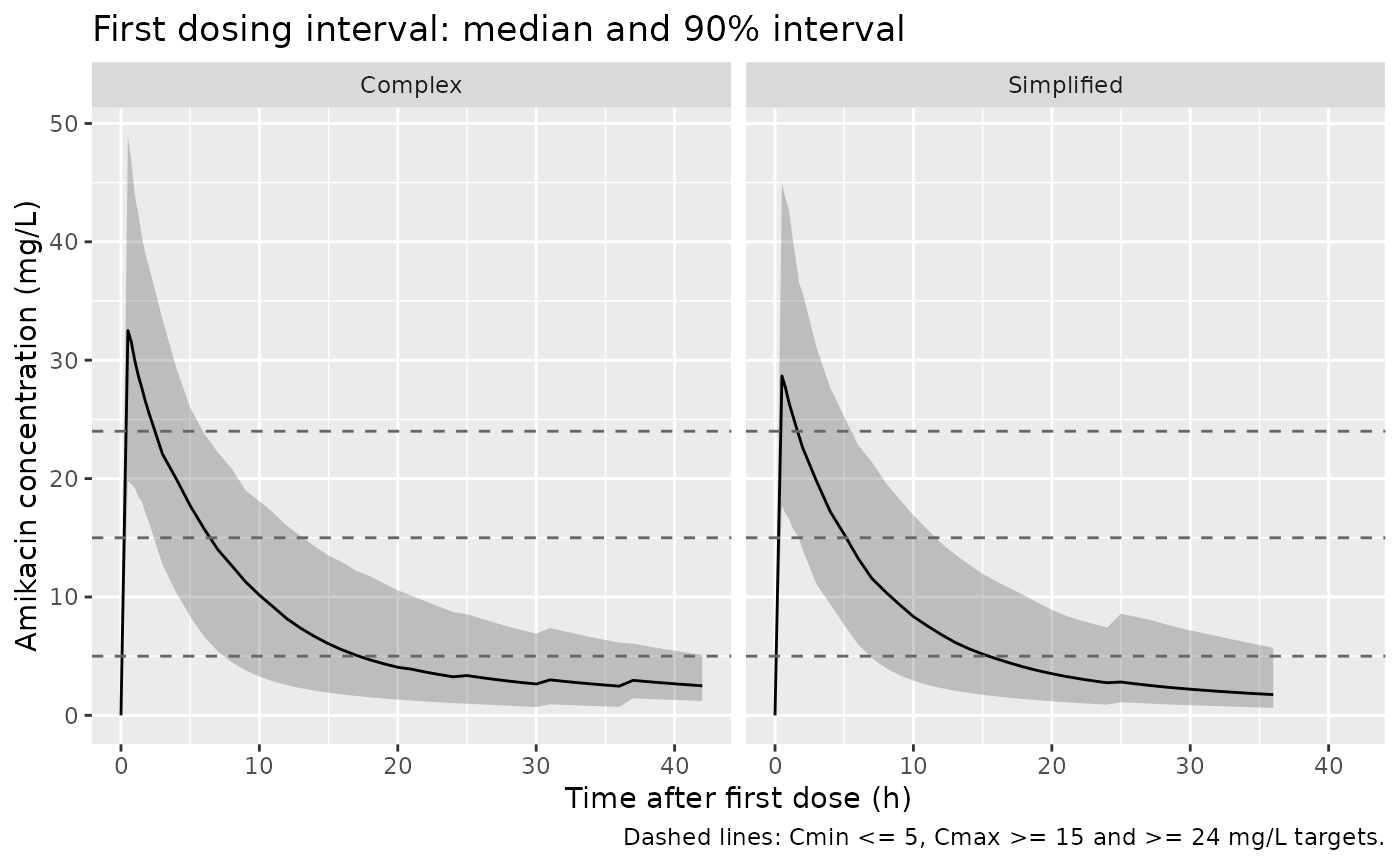
Each neonate receives one dose as a 30-minute infusion and is followed to the end of its first dosing interval, as in the paper’s target-attainment analysis. Cmax is the concentration 1 hour after the start of the infusion and Cmin the concentration just before the second dose (Methods ‘Evaluation of target attainment’).
mod <- readModelDb("vanderVeer_2025_amikacin")

obs_times <- function(tau) sort(unique(c(seq(0, 2, by = 0.25), seq(3, tau, by = 1), tau)))

doses <- cohort |>
  mutate(time = 0, evid = 1L, amt = dose, rate = dose / 0.5, cmt = "central")
obs <- cohort |>
  rowwise() |>
  reframe(id = id, time = obs_times(tau)) |>
  left_join(cohort, by = "id") |>
  mutate(evid = 0L, amt = 0, rate = 0, cmt = "central")
events <- bind_rows(doses, obs) |>
  arrange(id, time, desc(evid)) |>
  select(id, time, evid, amt, rate, cmt, regimen, tau, WT, WT_BIRTH, PNA)

sim <- rxode2::rxSolve(
  mod,
  events = events,
  keep = c("regimen", "tau"),
  returnType = "data.frame"
) |>
  filter(!is.na(Cc))
#> ℹ parameter labels from comments will be replaced by 'label()'
stopifnot(all(sim$Cc >= -1e-6 * max(sim$Cc)))
sim |>
  group_by(regimen, time) |>
  filter(n() >= 20) |>
  summarise(
    Q05 = quantile(Cc, 0.05),
    Q50 = median(Cc),
    Q95 = quantile(Cc, 0.95),
    .groups = "drop"
  ) |>
  ggplot(aes(time, Q50)) +
  geom_ribbon(aes(ymin = Q05, ymax = Q95), alpha = 0.25) +
  geom_line() +
  geom_hline(yintercept = c(5, 15, 24), linetype = "dashed", colour = "grey40") +
  facet_wrap(~regimen) +
  labs(
    x = "Time after first dose (h)", y = "Amikacin concentration (mg/L)",
    title = "First dosing interval: median and 90% interval",
    caption = "Dashed lines: Cmin <= 5, Cmax >= 15 and >= 24 mg/L targets."
  )
PKNCA: Cmin and AUC over the first dosing interval
PKNCA computes the trough at the end of each neonate’s first interval and the AUC over it; the 1-hour Cmax is read from the simulation directly because it is defined at a fixed time, not as the observed maximum.
sim_nca <- sim |>
  select(id, time, Cc, regimen) |>
  mutate(Cc = pmax(Cc, 0))
dose_df <- doses |> select(id, time, amt, regimen)

conc_obj <- PKNCA::PKNCAconc(sim_nca, Cc ~ time | regimen + id)
dose_obj <- PKNCA::PKNCAdose(dose_df, amt ~ time | regimen + id)
intervals <- cohort |>
  transmute(
    regimen, id,
    start = 0, end = tau, auclast = TRUE, ctrough = TRUE
  )
nca_res <- PKNCA::pk.nca(PKNCA::PKNCAdata(conc_obj, dose_obj, intervals = intervals))

nca_wide <- as.data.frame(nca_res) |>
  filter(PPTESTCD %in% c("auclast", "ctrough")) |>
  select(id, regimen, PPTESTCD, PPORRES) |>
  pivot_wider(names_from = PPTESTCD, values_from = PPORRES)

cmax_1h <- sim |>
  filter(abs(time - 1) < 1e-8) |>
  select(id, cmax1h = Cc)

exposure <- nca_wide |>
  inner_join(cmax_1h, by = "id")
stopifnot(
  nrow(exposure) == nrow(cohort),
  !anyNA(exposure$auclast), !anyNA(exposure$ctrough)
)
Replicate Figure 1: target attainment after the first dose
Figure 1 of the paper reports, for all neonates in each cohort, the percentage reaching each target, computed from the individual Bayesian estimates of the optimized model. The virtual cohorts below are drawn from the population model instead, so close but not exact agreement is expected.
mic <- c(2, 4, 8)
target_attainment <- exposure |>
  group_by(regimen) |>
  summarise(
    `Cmax >= 15 mg/L` = 100 * mean(cmax1h >= 15),
    `Cmax >= 24 mg/L` = 100 * mean(cmax1h >= 24),
    `Cmax >= 35 mg/L` = 100 * mean(cmax1h >= 35),
    `Cmin <= 3 mg/L` = 100 * mean(ctrough <= 3),
    `Cmin <= 5 mg/L` = 100 * mean(ctrough <= 5),
    `AUC/MIC >= 21.4, MIC 2` = 100 * mean(auclast / 2 >= 21.4),
    `AUC/MIC >= 21.4, MIC 4` = 100 * mean(auclast / 4 >= 21.4),
    `AUC/MIC >= 21.4, MIC 8` = 100 * mean(auclast / 8 >= 21.4),
    `AUC/MIC >= 62.5, MIC 2` = 100 * mean(auclast / 2 >= 62.5),
    `AUC/MIC >= 62.5, MIC 4` = 100 * mean(auclast / 4 >= 62.5),
    `AUC/MIC >= 62.5, MIC 8` = 100 * mean(auclast / 8 >= 62.5),
    .groups = "drop"
  ) |>
  pivot_longer(-regimen, names_to = "Target", values_to = "Simulated")

# Figure 1, rows 'All neonates' of each regimen.
published <- tibble::tribble(
  ~Target, ~Simplified, ~Complex,
  "Cmax >= 15 mg/L", 100, 100,
  "Cmax >= 24 mg/L", 88, 94,
  "Cmax >= 35 mg/L", 8, 1,
  "Cmin <= 3 mg/L", 82, 60,
  "Cmin <= 5 mg/L", 97, 94,
  "AUC/MIC >= 21.4, MIC 2", 100, 100,
  "AUC/MIC >= 21.4, MIC 4", 100, 100,
  "AUC/MIC >= 21.4, MIC 8", 94, 99,
  "AUC/MIC >= 62.5, MIC 2", 99, 99,
  "AUC/MIC >= 62.5, MIC 4", 53, 82,
  "AUC/MIC >= 62.5, MIC 8", 1, 4
) |>
  pivot_longer(-Target, names_to = "regimen", values_to = "Published")

ta_cmp <- inner_join(published, target_attainment, by = c("Target", "regimen")) |>
  mutate(Difference = Simulated - Published)
stopifnot(nrow(ta_cmp) == nrow(published))

ta_cmp |>
  rename(Regimen = regimen, `Published (%)` = Published, `Simulated (%)` = Simulated) |>
  knitr::kable(
    digits = 0,
    caption = "Target attainment (%) over the first dosing interval: Figure 1 ('All neonates') vs. the virtual cohorts."
)| Target | Regimen | Published (%) | Simulated (%) | Difference |
|---|---|---|---|---|
| Cmax >= 15 mg/L | Simplified | 100 | 97 | -3 |
| Cmax >= 15 mg/L | Complex | 100 | 99 | -1 |
| Cmax >= 24 mg/L | Simplified | 88 | 64 | -24 |
| Cmax >= 24 mg/L | Complex | 94 | 82 | -12 |
| Cmax >= 35 mg/L | Simplified | 8 | 16 | 8 |
| Cmax >= 35 mg/L | Complex | 1 | 24 | 24 |
| Cmin <= 3 mg/L | Simplified | 82 | 72 | -10 |
| Cmin <= 3 mg/L | Complex | 60 | 62 | 2 |
| Cmin <= 5 mg/L | Simplified | 97 | 90 | -6 |
| Cmin <= 5 mg/L | Complex | 94 | 93 | -1 |
| AUC/MIC >= 21.4, MIC 2 | Simplified | 100 | 100 | 0 |
| AUC/MIC >= 21.4, MIC 2 | Complex | 100 | 100 | 0 |
| AUC/MIC >= 21.4, MIC 4 | Simplified | 100 | 100 | 0 |
| AUC/MIC >= 21.4, MIC 4 | Complex | 100 | 100 | 0 |
| AUC/MIC >= 21.4, MIC 8 | Simplified | 94 | 82 | -12 |
| AUC/MIC >= 21.4, MIC 8 | Complex | 99 | 87 | -12 |
| AUC/MIC >= 62.5, MIC 2 | Simplified | 99 | 94 | -5 |
| AUC/MIC >= 62.5, MIC 2 | Complex | 99 | 96 | -4 |
| AUC/MIC >= 62.5, MIC 4 | Simplified | 53 | 47 | -6 |
| AUC/MIC >= 62.5, MIC 4 | Complex | 82 | 62 | -20 |
| AUC/MIC >= 62.5, MIC 8 | Simplified | 1 | 2 | 2 |
| AUC/MIC >= 62.5, MIC 8 | Complex | 4 | 6 | 2 |
ta_cmp |>
  ggplot(aes(Published, Simulated, colour = regimen)) +
  geom_abline(linetype = "dashed") +
  geom_point(size = 2) +
  coord_equal(xlim = c(0, 100), ylim = c(0, 100)) +
  labs(
    x = "Published target attainment (%)", y = "Simulated target attainment (%)",
    colour = "Regimen",
    caption = "Replicates the 'All neonates' rows of Figure 1 of van der Veer 2025."
  )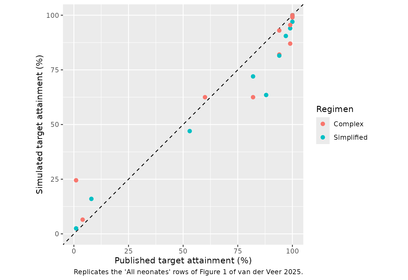
The targets near the centre of the exposure distributions agree to within a few percentage points (Cmin <= 3 and <= 5 mg/L, Cmax >= 15 mg/L, AUC/MIC at MIC 2 and 4 mg/L for the simplified regimen). The targets in the tails do not: the simulation places more neonates both below 24 mg/L and above 35 mg/L than Figure 1, and fewer above the AUC/MIC thresholds at MIC 8 mg/L. The published Cmax distribution is very narrow (94% of the complex-regimen neonates at or above 24 mg/L and 1% at or above 35 mg/L). The likely reason is that Figure 1 is built from empirical Bayes estimates. With one or two samples per neonate, the individual central-volume estimates shrink towards the typical value, while the population simulation draws the full 30% IIV on V1. The centres agree: the median simulated 1-hour Cmax is between 24 and 35 mg/L in both cohorts, the interval that holds at least 93% of the published neonates.
exposure |>
  group_by(regimen) |>
  summarise(
    `Cmax 1 h, median (mg/L)` = median(cmax1h),
    `Cmin, median (mg/L)` = median(ctrough),
    `AUC0-tau, median (mg*h/L)` = median(auclast),
    .groups = "drop"
  ) |>
  rename(Regimen = regimen) |>
knitr::kable(digits = 1, caption = "Simulated first-interval exposure (medians).")| Regimen | Cmax 1 h, median (mg/L) | Cmin, median (mg/L) | AUC0-tau, median (mg*h/L) |
|---|---|---|---|
| Complex | 30.0 | 2.4 | 282.6 |
| Simplified | 26.4 | 2.1 | 241.8 |
The gates below check the clinically used targets that the paper reports as met in at least 90% of neonates with both regimens: Cmax >= 15 mg/L, Cmin <= 5 mg/L and the bacteriostatic AUC/MIC at MIC 4 mg/L. They also check the median 1-hour Cmax and the median absolute difference across all 22 cells. A misread volume moves the Cmax rows by tens of percentage points, and a misread clearance or PNA coefficient moves the Cmin and AUC rows. Over three seeds the simulation gave 97-100, 90-93 and 98-100% for the three targets, medians of 26.4-30.0 mg/L, and median absolute differences of about 6 percentage points. Every bound sits at least three binomial standard errors (3.5 percentage points at p = 0.5 with 200 neonates) away from those values.
ta_val <- function(target, reg) {
  v <- ta_cmp$Simulated[ta_cmp$Target == target & ta_cmp$regimen == reg]
  if (length(v) != 1L) stop("no unique row for '", target, "' / ", reg)
  v
}
for (reg in c("Simplified", "Complex")) {
  cmax_med <- median(exposure$cmax1h[exposure$regimen == reg])
  stopifnot(
    ta_val("Cmax >= 15 mg/L", reg) >= 85,
    ta_val("Cmin <= 5 mg/L", reg) >= 80,
    ta_val("AUC/MIC >= 21.4, MIC 4", reg) >= 85,
    cmax_med > 22, cmax_med < 35
  )
}
stopifnot(median(abs(ta_cmp$Difference)) < 12)
Typical-value check: AUC = dose / CL
For the reference neonate of Table S5 (birth weight 1685 g, current weight 1700 g, postnatal age 5 days) the paper’s equation gives CL = 0.044 x (1 + 0.597 x 5/5) = 0.0703 L/h. The AUC to infinity of a single dose computed by PKNCA from the typical-value solve must equal dose / CL.
cl_ref <- 0.044 * (1.685 / 1.685)^1.34 * (1 + 0.597 * 5 / 5)
ref_ev <- tibble(
  id = 1L, WT_BIRTH = 1.685, WT = 1.700, PNA = 5 / 30.4375
)
dose_ref <- 15 * 1.700
ev_ref <- bind_rows(
  ref_ev |> mutate(time = 0, evid = 1L, amt = dose_ref, rate = dose_ref / 0.5, cmt = "central"),
  ref_ev |> reframe(id, WT_BIRTH, WT, PNA, time = c(seq(0, 2, by = 0.05), seq(2.5, 400, by = 0.5))) |>
    mutate(evid = 0L, amt = 0, rate = 0, cmt = "central")
) |>
  arrange(time, desc(evid))

sim_ref <- rxode2::rxSolve(
  rxode2::zeroRe(mod), events = ev_ref, rtol = 1e-10, atol = 1e-12,
  returnType = "data.frame"
) |>
  filter(!is.na(Cc)) |>
  mutate(id = 1L, Cc = pmax(Cc, 0), regimen = "reference")
#> ℹ parameter labels from comments will be replaced by 'label()'
#> ℹ omega/sigma items treated as zero: 'etalcl', 'etalvc'

nca_ref <- PKNCA::pk.nca(PKNCA::PKNCAdata(
  PKNCA::PKNCAconc(sim_ref, Cc ~ time | regimen + id),
  PKNCA::PKNCAdose(
    ev_ref |> filter(evid == 1) |> mutate(regimen = "reference"),
    amt ~ time | regimen + id
  ),
  intervals = data.frame(start = 0, end = Inf, aucinf.obs = TRUE)
))
auc_ref <- as.data.frame(nca_ref) |>
  filter(PPTESTCD == "aucinf.obs") |>
  pull(PPORRES)

knitr::kable(
  tibble(
    Quantity = c("CL from Table S5 (L/h)", "Dose (mg)", "Dose / CL (mg*h/L)", "PKNCA AUC0-inf (mg*h/L)"),
    Value = c(cl_ref, dose_ref, dose_ref / cl_ref, auc_ref)
  ),
  digits = 4
)| Quantity | Value |
|---|---|
| CL from Table S5 (L/h) | 0.0703 |
| Dose (mg) | 25.5000 |
| Dose / CL (mg*h/L) | 362.8963 |
| PKNCA AUC0-inf (mg*h/L) | 362.9098 |
Assumptions and deviations
-
Residual error and IIV scale. Table S5 gives the
variability terms without stating their scale. The “IIV on V1” entry is
0.09 for the 30% CV that the text says was fixed (0.3^2), so the table
reports NONMEM variances; the residual-error entries are read the same
way (proportional 0.0279 -> SD 16.7%, additive 0.378 -> SD 0.615
mg/L). Read as standard deviations, the proportional term would be 2.8%,
below the < 5% precision of the assays themselves. The combined error
is encoded as variance-additive
(
add(addSd) + prop(propSd)), the NONMEMF + F*EPS(1) + EPS(2)form. - Q = r x CL. The table writes Q as a fraction of CL; the model applies it to the individual CL (including its random effect and covariates).
-
Ibuprofen. The De Cock 2012 ibuprofen factor (0.838
on CL) equals 1 in the optimized model (Table S5 footnote c), so the
ibuprofen co-medication indicator is documented in
covariatesDataExcludedbut not used. - Covariate centring. Birth weight, current weight and postnatal age are centred on the pooled model-building medians in Table S5 footnote b (1685 g, 1700 g, 5 days), not the De Cock 2012 medians (1750 g, 1760 g, 2 days).
- Virtual cohorts. Gestational and postnatal age come from piecewise-linear quantile functions through the Table 3 and Table S1 summary points; birth weight from an approximate median birth-weight-for-gestational-age curve with 15% scatter, rescaled to the Table 3 medians; current weight from birth weight with 5% scatter. The infusion duration is 30 minutes (the paper gives 20-30 minutes). The complex regimen omits the 10-hour ibuprofen prolongation and the optional 6-hour prolongation for groups 7 and 9, as the paper did.
- Figure 1 comparison. The paper’s percentages come from individual Bayesian estimates for the observed neonates; the comparison here uses population simulations of approximate cohorts. Centre-of-distribution targets agree to within a few percentage points; tail targets (Cmax >= 24 and >= 35 mg/L, AUC/MIC at MIC 8 mg/L, AUC/MIC >= 62.5 at MIC 4 mg/L for the complex regimen) differ by 10-30 percentage points, which is consistent with shrinkage of the individual estimates (see the Figure 1 section).
- Models not packaged. Table S3 (De Cock 2012 parameters re-estimated on the Amsterdam data alone) is an external-validation diagnostic, and the original De Cock 2012 parameters belong to that earlier publication; neither is the paper’s final model.
- Errata. No correction notice was found in Europe PMC as of 2026-11-03.