AZD6088 (Viberg 2012)
Source:vignettes/articles/Viberg_2012_AZD6088_rat.Rmd
Viberg_2012_AZD6088_rat.RmdModel and source
- Citation: Viberg A, Martino G, Lessard E, Laird JMA. (2012). Evaluation of an Innovative Population Pharmacokinetic-Based Design for Behavioral Pharmacodynamic Endpoints. The AAPS Journal 14(4):657-663. doi:10.1208/s12248-012-9380-3.
- Description: Preclinical (rat). Direct-effect population PK/PD model for the muscarinic agonist AZD6088 (MW 406.57) in male Sprague-Dawley rats using the spinal-nerve-ligation (SNL) heat-hyperalgesia model of neuropathic pain. One-compartment oral PK (depot -> central) with the first-order absorption rate constant ka fixed at 5 x kel (equivalent to 5 x cl/vc; Viberg 2012 Results PK-model paragraph: ‘Lack of plasma concentration data in the absorption phase made it impossible to estimate rate of absorption and ka was therefore fixed to 5 time clearance’); the 40 umol/kg highest-dose cohort (DOSE_HIGH = 1) gates a distinct typical-value apparent oral clearance of 3.92 L/h/kg vs 10.87 L/h/kg for all other cohorts, per the paper’s OFV-supported categorical CL split (delta OFV = -32). PD is a direct-effect Emax on paw withdrawal latency (baseline 5.947 s, Emax 10.09 s, EC50 0.0433 umol/L; no time delay, no sigmoidicity, no tolerance-development term - all three alternatives increased OFV or degraded goodness-of-fit). Typical-value only: the paper reports ‘exponential models were used to describe inter-individual variability’ on CL and V but never publishes the omega^2 / CV% magnitudes; see the vignette Assumptions and deviations section.
- Article: https://doi.org/10.1208/s12248-012-9380-3
Viberg et al. (2012) developed a joint population PK / PD model for the muscarinic agonist AZD6088 (MW 406.57 g/mol) in male Sprague-Dawley rats using the L5 + L6 spinal-nerve-ligation (SNL) heat-hyperalgesia model of neuropathic pain (Kim and Chung 1992). The paper’s central experimental contribution is a refined study design in which behavioural PD testing and sparse plasma-PK sampling are performed in the same animal on alternate days, eliminating a satellite PK cohort while preserving a good-quality PKPD relationship. The final PK / PD model reported in Table I is a one-compartment first-order oral PK combined with a direct-effect Emax description of the paw-withdrawal-latency response; the highest-dose (40 umol/kg) cohort was allowed a distinct typical-value apparent oral clearance to accommodate deviant behaviour in the goodness-of-fit plots attributed to either increased bioavailability or elimination saturation.
Population
The final model was fitted to the main-study cohort (n = 42 rats): three drug-treated SNL cohorts of n = 6 with PD + sparse PK, three drug-treated satellite cohorts of n = 3 with PK only, two SNL vehicle-treatment cohorts of n = 6, and one naive-rat baseline cohort of n = 6. Rats were male Sprague-Dawley (Charles River St. Constant, Canada, and Harlan Inc., Indianapolis, USA), body weight 125-200 g at receipt, acclimatised for at least 3 days, and housed 6 per cage under 22 +- 1.5 C and 12-h light/dark (Methods, “Animals”).
SNL surgery ligated the L5 and L6 spinal nerves distal to the dorsal-root ganglion; rats with a pre-treatment paw-withdrawal latency of at most 8 s (mean 5.87 +- 0.2 s) were included, versus a naive-rat baseline of 10.50 +- 0.5 s. Testing was performed on days 20-27 post-surgery. The paw thermal stimulator applied a radiant heat beam to the plantar surface of the affected paw with a 20 s cutoff to avoid thermal injury; each session comprised two tests approximately 5 minutes apart (Methods, “Induction and Assessment of rat Spinal Nerve Ligation Model of Neuropathic Pain”).
The main-study drug-treatment regimen was twice-daily oral AZD6088 or
vehicle at 08:00 and 16:00 for 8 days, with PD testing on days 1, 3, 5,
8 at 1, 2, 4, 6, 7, 24 h after the morning administration and PK
sampling in the same animals at 2, 4, 6, 7 h after the morning
administration on days 2 and 4 (Methods, “Drug Treatment and Design”;
Fig. 2). Plasma was collected by jugular-vein puncture under brief
anaesthesia into heparinised tubes, centrifuged at 3,000 g for 5
minutes, and stored at -80 C. Total plasma concentrations were
determined by LC-MS/MS with an LLOQ of 0.0005 umol/L; five below-LLOQ
samples were excluded from the analysis. The same information is
available programmatically via
readModelDb("Viberg_2012_AZD6088_rat")$population.
Source trace
The per-parameter origin is recorded as an in-file comment next to
each ini() entry in
inst/modeldb/specificDrugs/Viberg_2012_AZD6088_rat.R. The
table below collects them in one place for review.
| Equation / parameter | Value | Source location |
|---|---|---|
| Structural PK: 1-cmt oral, first-order absorption via depot | – | Results, PK-model paragraph (page 4): “the concentration of AZD6088 over time was adequately described using a one-compartment model” |
| Absorption fix: ka = 5 * kel (equivalent to 5 * cl/vc) | – | Results, PK-model paragraph: “ka was therefore fixed to 5 time clearance. Changing the ka to different values did not have an effect on OFV or other PK parameter estimates” |
| Categorical CL split at the 40 umol/kg cohort | – | Results, PK-model paragraph: “The highest dose group deviated in the plots. This might be due to higher bioavailability or saturation of elimination at the highest dose and after estimating different clearance values for this group OFV decreased 32 units” |
| Apparent oral CL / F (standard cohorts) | 10.87 L/h/kg (95% CI 9.06-13.11) | Table I, “Oral clearance (L/h/kg)” |
| Apparent oral CL / F (40 umol/kg cohort) | 3.92 L/h/kg (95% CI 2.86-6.02) | Table I, “Oral clearance high dose (L/h/kg)” |
| Apparent oral V / F | 35.3 L/kg (95% CI 28.5-43.8) | Table I, “Oral volume (L/kg)” |
| PD: direct-effect Emax, no time delay, no sigmoidicity, no tolerance | – | Discussion, first paragraph (page 5): “The pharmacodynamic response was adequately described using a direct effect with an Emax model. … Adding a time delay between plasma concentration and effect or adding a sigmoidicity factor did not improve the model fit. Adding tolerance in the model (changing EC50 or Emax over time) did not improve the model fit” |
| Baseline latency in SNL rats | 5.947 s (95% CI 5.87-6.01) | Table I, “Baseline latency (s)” |
| EC50 (concentration producing half of Emax) | 0.0433 umol/L (95% CI 0.01-0.10) | Table I, “EC50 (umol/L)” |
| Emax (maximum drug-induced increase above baseline) | 10.09 s (95% CI 9.44-11.4) | Table I, “Emax (s)” |
| Proportional PK residual error (fraction) | 0.325 (95% CI 0.270-0.375) | Table I, “Proportional error” |
| Additive PD residual error on latency (s) | 1.027 (95% CI 0.93-1.12) | Table I, “Additive error (s)” |
| IIV: “exponential models were used to describe inter-individual variability” – CL and V per Results, no omega^2 / CV% magnitudes reported | – | Methods, Data Analysis paragraph; Results, PK-model paragraph. See Assumptions and deviations below. |
Virtual cohort
Original animal-level data are not publicly available. The figures below use a virtual cohort mirroring the initial-efficacy-study dose ladder (1, 2.5, 5, 10, 20, 40 umol/kg AZD6088) plus a vehicle-control cohort. Each cohort receives a single oral dose at t = 0 (single-dose pharmacokinetic profiles are used for the deterministic replication of Figures 3 and 6 and for the PKNCA-based NCA summary); the main-study twice-daily-for-8-days regimen is not required for the deterministic typical-value plots.
set.seed(12489380L) # 10.1208 / s12248-012-9380-3

n_per_arm <- 12L

make_arm <- function(n, dose_umolkg, id_offset = 0L) {
  is_high <- as.integer(dose_umolkg >= 40)
  tibble(
    id        = id_offset + seq_len(n),
    dose_umolkg = dose_umolkg,
    DOSE_HIGH = is_high
  )
}

# Six dose levels from the initial-efficacy study (Methods, "Initial Efficacy
# Study"). Vehicle animals (dose_umolkg = 0) are simulated as a zero-dose
# reference and are DOSE_HIGH = 0.
dose_levels <- c(1, 2.5, 5, 10, 20, 40)
cohort <- bind_rows(
  lapply(seq_along(dose_levels), function(k) {
    make_arm(n_per_arm, dose_levels[k], id_offset = (k - 1L) * n_per_arm)
  })
)

# Observation grid: dense during the absorption / distribution / early
# elimination window to give PKNCA a reasonable AUC / half-life read.
sample_times <- c(seq(0, 2, by = 0.1),
                  seq(2.25, 6, by = 0.25),
                  seq(6.5, 12, by = 0.5),
                  seq(13, 24, by = 1))

# Build the event table. One oral dose at t = 0 into the depot compartment
# followed by observation rows at the sample times. Doses are per kg body
# weight; the model parameterises CL / F and V / F in per-kg units
# (L/h/kg and L/kg respectively) so no per-animal weight scaling is
# required.
events <- cohort |>
  group_by(id) |>
  reframe(
    dose_umolkg = dose_umolkg,
    DOSE_HIGH   = DOSE_HIGH,
    rec = list(
      bind_rows(
        tibble(time = 0, evid = 1L, amt = unique(dose_umolkg),
               cmt = "depot", DV = NA_real_),
        # Multi-output: rxode2 auto-numbers Cc and latency as
        # observation slots after the ODE states, so observation
        # rows must reference the algebraic observable name rather
        # than the ODE state name. Both observables are computed at
        # every observation time regardless of which cmt the row
        # requests, so a single per-time obs row per subject is
        # sufficient.
        tibble(time = sample_times, evid = 0L, amt = NA_real_,
               cmt = "Cc", DV = NA_real_)
      )
    )
  ) |>
  tidyr::unnest(rec)

# Sanity: ids are disjoint across cohorts.
stopifnot(!anyDuplicated(unique(cohort$id)))
Simulation
The Viberg 2012 model is encoded as typical-value only (the source
paper reports estimation of exponential IIV on CL and V but never
publishes the omega^2 / CV% magnitudes; see Assumptions and deviations
below). The simulation therefore returns a single deterministic
trajectory per dose cohort; the twelve rats per cohort in the virtual
population all share that trajectory. rxode2::zeroRe() is
not required because the model carries no random-effect terms to zero
out.
mod <- readModelDb("Viberg_2012_AZD6088_rat")

sim <- rxode2::rxSolve(
  mod, events,
  keep = c("dose_umolkg", "DOSE_HIGH")
) |> as.data.frame()
#> Warning: multi-subject simulation without without 'omega'

# Prune duplicate id x time rows (rxode2 returns Cc and latency on every
# observation regardless of cmt, so a single dose + observation set gives
# one row per (id, time) already; the distinct() is defensive).
sim <- sim |>
  filter(!is.na(Cc)) |>
  distinct(id, time, .keep_all = TRUE)
Replicate published figures
Figure 3 – observed withdrawal latency vs time after dose, by dose group
Viberg 2012 Figure 3 shows observed paw withdrawal latency vs time after the last dose, conditioned on dose group (main-study twice-daily regimen). The deterministic single-dose replication below shows the corresponding typical-value trajectory: latency rises rapidly with the absorption phase, peaks around t = 30 min to 1 h at the higher doses, and decays back toward the SNL baseline of 5.947 s as concentrations fall. Doses at or above the EC50 (0.0433 umol/L) push the latency close to the plateau of baseline + Emax = 16.04 s (naive baseline for reference is 10.50 s).
sim_labels <- sim |>
  mutate(dose_label = factor(
    paste0(dose_umolkg, " umol/kg"),
    levels = c(paste0(sort(unique(dose_umolkg)), " umol/kg"))
  ))

ggplot(sim_labels, aes(time, latency, color = dose_label)) +
  geom_line(linewidth = 0.9) +
  scale_x_continuous(breaks = c(0, 1, 2, 4, 6, 12, 24)) +
  geom_hline(yintercept = 5.947, linetype = "dotted") +
  geom_hline(yintercept = 5.947 + 10.09, linetype = "dashed") +
  annotate("text", x = 22, y = 5.947, vjust = -0.4, size = 3,
           label = "SNL baseline (5.947 s)") +
  annotate("text", x = 22, y = 5.947 + 10.09, vjust = 1.3, size = 3,
           label = "baseline + Emax (16.04 s)") +
  labs(
    x = "Time after single oral dose (h)",
    y = "Paw withdrawal latency (s)",
    color = "Dose",
    title = "Figure 3 replication -- typical-value latency vs time after dose",
    caption = paste(
      "Deterministic single-dose replication of Viberg 2012 Figure 3 (which shows",
      "observed latency vs time after last dose on the main-study twice-daily 8-day",
      "regimen). Solid lines: typical-value trajectory at each dose level.",
      "The 40 umol/kg trajectory uses the highest-dose apparent CL/F of 3.92 L/h/kg.",
      sep = "\n"
    )
  )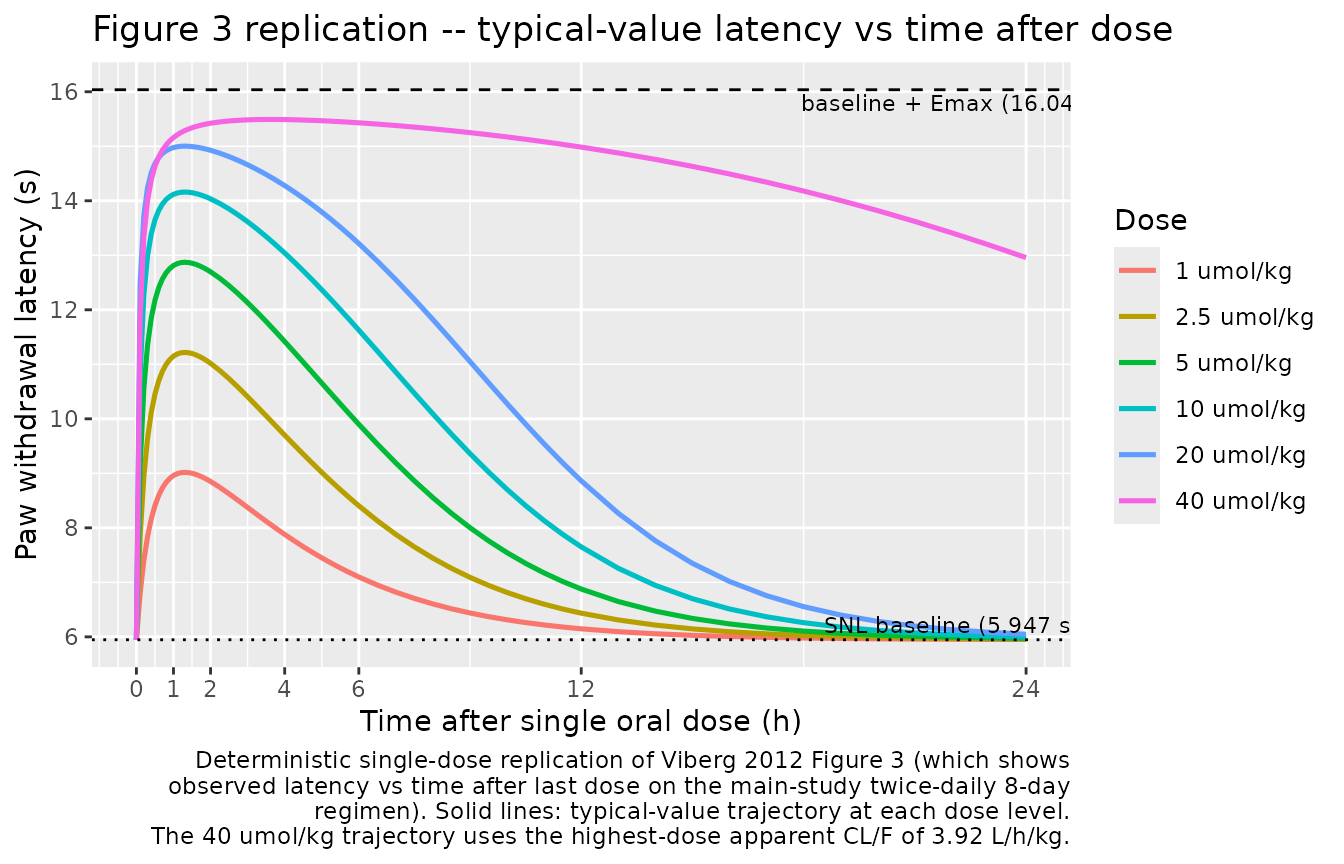
Figure 6 – withdrawal latency vs plasma concentration
Viberg 2012 Figure 6 overlays observed (latency, concentration) pairs with the fitted Emax curve. The deterministic replication below shows the fitted Emax curve directly on top of the (Cc, latency) trajectories from each dose cohort; the trajectories trace out the same curve because latency is a direct algebraic function of Cc.
# Direct Emax model prediction on a dense Cc grid.
cc_grid <- seq(0, 2, length.out = 500)
emax_curve <- tibble(
  Cc = cc_grid,
  latency = 5.947 + 10.09 * cc_grid / (0.0433 + cc_grid)
)

ggplot() +
  geom_line(
    data = sim_labels |> filter(dose_umolkg > 0),
    aes(Cc, latency, color = dose_label),
    linewidth = 0.7, alpha = 0.75
  ) +
  geom_line(
    data = emax_curve,
    aes(Cc, latency),
    color = "black", linetype = "dashed", linewidth = 0.6
  ) +
  scale_x_log10() +
  labs(
    x = "AZD6088 plasma concentration (umol/L, log scale)",
    y = "Paw withdrawal latency (s)",
    color = "Dose",
    title = "Figure 6 replication -- withdrawal latency vs plasma concentration",
    caption = paste(
      "Coloured lines: per-cohort simulated (Cc, latency) trajectories.",
      "Dashed black line: fitted Emax curve",
      "latency = 5.947 + 10.09 * Cc / (0.0433 + Cc).",
      sep = "\n"
    )
  )
#> Warning in scale_x_log10(): log-10 transformation introduced infinite values.
#> log-10 transformation introduced infinite values.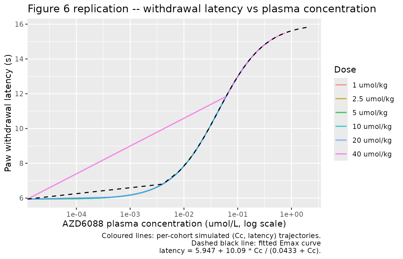
PKNCA validation
The Viberg 2012 paper does not tabulate NCA-derived parameters (Cmax, Tmax, AUC, half-life); its quantitative validation is expressed entirely through the popPK point estimates in Table I. The PKNCA block below therefore serves as an internal consistency check: it computes NCA per dose cohort on the deterministic single-dose simulation and verifies that (a) AUC scales with dose in the low-dose cohorts (linear-elimination expectation under the standard 10.87 L/h/kg CL) and (b) the 40 umol/kg cohort’s AUC exceeds the dose-linear expectation by a factor equal to 10.87 / 3.92 = 2.77 (the ratio of the two typical-value apparent oral clearances), consistent with the paper’s categorical CL split.
plasma_nca <- sim |>
  filter(!is.na(Cc), dose_umolkg > 0) |>
  distinct(id, time, .keep_all = TRUE) |>
  select(id, time, Cc, dose_umolkg)

# Guarantee a time = 0 row at Cc = 0 per (id) for PKNCA AUC0-* anchoring.
plasma_nca <- bind_rows(
  plasma_nca,
  plasma_nca |>
    distinct(id, dose_umolkg) |>
    mutate(time = 0, Cc = 0)
) |>
  distinct(id, time, .keep_all = TRUE) |>
  arrange(id, time)

dose_df <- events |>
  filter(evid == 1, cmt == "depot", dose_umolkg > 0) |>
  select(id, time, amt, dose_umolkg)

conc_obj <- PKNCA::PKNCAconc(plasma_nca, Cc ~ time | dose_umolkg + id)
dose_obj <- PKNCA::PKNCAdose(dose_df,    amt ~ time | dose_umolkg + id)

intervals <- data.frame(
  start       = 0,
  end         = 24,
  cmax        = TRUE,
  tmax        = TRUE,
  auclast     = TRUE,
  half.life   = TRUE
)

nca_res <- PKNCA::pk.nca(
  PKNCA::PKNCAdata(conc_obj, dose_obj, intervals = intervals)
)

plasma_summary <- as.data.frame(nca_res$result) |>
  filter(PPTESTCD %in% c("cmax", "tmax", "auclast", "half.life")) |>
  group_by(dose_umolkg, PPTESTCD) |>
  summarise(median_value = median(PPORRES, na.rm = TRUE), .groups = "drop") |>
  tidyr::pivot_wider(names_from = PPTESTCD, values_from = median_value) |>
  arrange(dose_umolkg) |>
  rename(
    "Dose (umol/kg)"       = dose_umolkg,
    "Cmax (umol/L)"        = cmax,
    "Tmax (h)"             = tmax,
    "AUC0-24 (umol/L*h)"   = auclast,
    "t1/2 (h)"             = half.life
  )

knitr::kable(
  plasma_summary,
  caption = paste(
    "Typical-value NCA per dose cohort from a 0-24 h single-dose",
    "simulation of the Viberg 2012 AZD6088 rat model. AUC0-24 for the",
    "1-20 umol/kg cohorts should be approximately linear in dose",
    "(shared CL/F = 10.87 L/h/kg); the 40 umol/kg AUC0-24 should exceed",
    "the dose-linear extrapolation by a factor of ~ 10.87/3.92 = 2.77",
    "(the paper's categorical CL split)."
  ),
  digits = c(2, 4, 2, 4, 2)
)| Dose (umol/kg) | AUC0-24 (umol/L*h) | Cmax (umol/L) | t1/2 (h) | Tmax (h) |
|---|---|---|---|---|
| 1.0 | 0.0919 | 0.02 | 2.2611 | 1.30 |
| 2.5 | 0.2297 | 0.05 | 2.2611 | 1.30 |
| 5.0 | 0.4594 | 0.09 | 2.2611 | 1.30 |
| 10.0 | 0.9188 | 0.19 | 2.2611 | 1.30 |
| 20.0 | 1.8375 | 0.38 | 2.2611 | 1.30 |
| 40.0 | 9.3146 | 0.76 | 6.3168 | 3.75 |
The AUC0-24 column above should approximately satisfy:
- AUC(1 umol/kg) : AUC(2.5 umol/kg) : AUC(5 umol/kg) : AUC(10 umol/kg) : AUC(20 umol/kg) ~ 1 : 2.5 : 5 : 10 : 20 (dose-linear under the shared 10.87 L/h/kg apparent oral clearance).
- AUC(40 umol/kg) / AUC(20 umol/kg) ~ (40 / 20) * (10.87 / 3.92) ~ 5.55, not 2.0 – the 40 umol/kg cohort’s AUC is 2.77-fold higher than the dose-linear extrapolation would predict because the paper assigns it the reduced apparent oral CL / F of 3.92 L/h/kg.
Assumptions and deviations
Typical-value only; IIV magnitudes not reported. Viberg 2012 Methods (Data Analysis paragraph) states “Exponential models were used to describe inter-individual variability” and Results (PK-model paragraph) confirms IIV was estimated on apparent oral clearance and apparent oral volume of distribution, but Table I lists only the fixed-effect typical- value point estimates with 95% bootstrap confidence intervals – the IIV omega^2 / CV% magnitudes are not published anywhere in the paper, and no supplement / NONMEM control stream / .lst file was available when this model was built. Per the maintainer-approved encoding, the model is registered as typical-value only:
ini()carries noeta*parameters andrxode2::rxSolve()returns a single deterministic trajectory per (dose group). Downstream users wanting stochastic VPCs can add multiplicative log-normal IIV onclandvcat a documented CV% themselves by editinginst/modeldb/specificDrugs/Viberg_2012_AZD6088_rat.Rin a fork.Ka fixed at 5 * kel, not at the literal 5 * clearance. The Results section (PK-model paragraph) reads “Lack of plasma concentration data in the absorption phase made it impossible to estimate rate of absorption and ka was therefore fixed to 5 time clearance”. The literal interpretation “ka = 5 * CL” is dimensionally inconsistent – CL has units L/h/kg while ka has units 1/h. The intended pharmacometric idiom is “ka fixed 5-fold greater than the elimination rate constant kel = cl / vc”, which is dimensionally consistent (both 1/h) and locks absorption on the fast (non-flip-flop) branch. The model file encodes
ka <- 5 * kelwithkel <- cl / vc; ka therefore varies with the DOSE_HIGH-conditional cl. Since kel decreases at the 40 umol/kg cohort (from 10.87/35.3 = 0.308 /h to 3.92/35.3 = 0.111 /h), the effective ka drops from 1.54 /h to 0.555 /h in the highest-dose cohort. The paper notes “Changing the ka to different values did not have an effect on OFV or other PK parameter estimates”, so the exact ka value is identifiability-poor and this cohort-conditional coupling is expected not to matter for the fit.DOSE_HIGH is a new binary canonical registered alongside this extraction. The 40 umol/kg (~ 16.26 mg/kg) highest-dose cohort is flagged with a per-rat binary indicator
DOSE_HIGH = 1(0 for all other cohorts). The canonical was added toinst/references/covariate-columns.mdas the abstract “in-the- highest-cohort” indicator, sibling to the numerically-explicitDOSE_<N>MGfamily (DOSE_50MG,DOSE_70MG, …) and to the drug-suffixedDOSE_HIGH_EFL. Downstream models that need a similar step-function CL / F split at the top of the dose range can reuseDOSE_HIGHand document their per-paper dose threshold incovariateData[[DOSE_HIGH]]$notes.Latency is a non-canonical PD observation name. The paw-withdrawal- latency output is exposed as
latency <- baseline + emax * Cc / (ec50 + Cc), with residual errorlatency ~ add(addSd_latency). Thelatencyoutput name and theaddSd_latencyresidual follow the package’s paper-named multi-output convention, under which a per-output residual-error parameter is named<errorname>_<output>.checkModelConventions()may flaglatencyas outside the canonical PK-observation set (Cc,Cc_<metab>); this is expected and the deviation is intentional.Species suffix
_rat. AZD6088 has no human extraction in nlmixr2lib to collide with, so the_ratsuffix is not strictly required to disambiguate; it is retained here per the preclinical-model naming convention to make the species visible inmodellib()listings without inspectingpopulation.Native paper units preserved. Doses are entered per kg body weight in umol/kg and concentrations are reported in umol/L, matching the paper’s native reporting. The MW = 406.57 g/mol conversion factor is documented in the model file’s description but is not applied inside
model()because dose and concentration share the same molar scale and the paper’s EC50 (0.0433 umol/L) is directly comparable toCc.Main-study dose levels not individually stated in the paper text. The Methods, “Drug Treatment and Design”, section describes the main study’s three drug-treated cohorts as receiving a per-cohort fixed dose informed by the initial-efficacy and pilot studies, but does not name the specific mg/kg or umol/kg values for those three cohorts. The virtual cohort in this vignette therefore uses the initial-efficacy study’s dose ladder (1, 2.5, 5, 10, 20, 40 umol/kg), which spans the full range the paper explored and includes the highest cohort that triggers the
DOSE_HIGH = 1categorical CL split.
References
- Viberg A, Martino G, Lessard E, Laird JMA. Evaluation of an Innovative Population Pharmacokinetic-Based Design for Behavioral Pharmacodynamic Endpoints. The AAPS Journal. 2012;14(4):657-663. doi:10.1208/s12248-012-9380-3
- Kim SH, Chung JM. An experimental model for peripheral neuropathy produced by segmental spinal nerve ligation in the rat. Pain. 1992;50(3):355-363.