Tacrolimus (Woillard 2011)
Source:vignettes/articles/Woillard_2011_tacrolimus.Rmd
Woillard_2011_tacrolimus.RmdModel and source
- Citation: Woillard JB, de Winter BCM, Kamar N, Marquet P, Rostaing L, Rousseau A. Population pharmacokinetic model and Bayesian estimator for two tacrolimus formulations – twice daily Prograf and once daily Advagraf. Br J Clin Pharmacol 2011; 71(3):391-402. doi:10.1111/j.1365-2125.2010.03837.x.
- Description: Two-compartment population PK model with Erlang-distributed transit absorption (3 transit compartments) for oral tacrolimus in adult renal transplant recipients pooled across the twice-daily immediate-release Prograf formulation and the once-daily prolonged-release Advagraf formulation (Woillard 2011), with multiplicative CYP3A5*1-carrier (expresser) and power-scaled haematocrit effects on apparent clearance, multiplicative formulation effects on the Erlang transit rate constant and on apparent central volume, and combined additive plus proportional residual error.
- Article: Br J Clin Pharmacol 2011;71(3):391-402. https://doi.org/10.1111/j.1365-2125.2010.03837.x
Population
The model was developed from two French pharmacokinetic trials in adult renal transplant recipients pooled into a single dataset of 73 patients and 186 PK profiles (Woillard 2011 Table 1). The Prograf cohort (n = 32; 145 profiles) consisted of de novo recipients sampled at weeks 1 and 2 and months 1, 3 and 6 post-transplant on twice-daily immediate-release tacrolimus titrated to a trough target of 10-15 ng/mL during the first 6 weeks and 5-10 ng/mL thereafter; concomitant mycophenolate mofetil and tapered oral prednisolone were given. The Advagraf cohort (n = 41; 41 profiles) consisted of stable recipients converted from cyclosporin A to once-daily prolonged-release tacrolimus at least 6 months before the study and sampled more than 12 months post-transplant. Median (range) age was 55 (18-69) years for Prograf and 53 (28-77) years for Advagraf, weight 65 (46-97) kg and 69 (45-116) kg, and haematocrit 32.3 % (20.9-46.6) and 38.5 % (26.5-45.1) respectively (Table 1). The CYP3A5 6986A>G genotype distribution across both cohorts was 1/1 = 1, 1/3 = 5, 3/3 = 67, giving 6 expressers and 67 nonexpressers. Tacrolimus was quantified in whole blood by validated turbulent-flow LC-MS/MS with a 1 ng/mL lower limit of quantification.
The same information is available programmatically via
readModelDb("Woillard_2011_tacrolimus")$population.
Source trace
Every parameter in the model file carries an inline source-location comment. The table below collects the entries in one place.
| Equation / parameter | Value | Source location |
|---|---|---|
lktr (Erlang transit rate Ktr for Advagraf reference,
theta1) |
3.34 1/h | Table 4 “Final model obtained in the whole dataset” column, Ktr row |
e_form_tac_ir_ktr (formulation multiplier on Ktr,
theta2) |
1.53 | Table 4 whole-dataset column, Ktr theta2 row |
lcl (CL/F for HCT = 35 %, CYP3A5 nonexpresser,
theta3) |
21.2 L/h | Table 4 whole-dataset column, CL/F theta3 row |
e_hct_cl (HCT power exponent on CL/F, theta4) |
-1.14 | Table 4 whole-dataset column, CL/F theta4 row |
e_cyp3a5_expr_cl (CYP3A5 multiplier on CL/F,
theta5) |
2.00 | Table 4 whole-dataset column, CL/F theta5 row |
lq (Q/F apparent inter-compartmental clearance) |
79 L/h | Table 4 whole-dataset column, Q/F row |
lvc (Vc/F for Advagraf reference, theta6) |
486 L | Table 4 whole-dataset column, Vc/F theta6 row |
e_form_tac_ir_vc (formulation multiplier on Vc/F,
theta7) |
0.29 | Table 4 whole-dataset column, Vc/F theta7 row |
lvp (Vp/F apparent peripheral volume) |
271 L | Table 4 whole-dataset column, Vp/F row |
| IIV Ktr (omega^2 = log(1 + 0.24^2) = 0.05605) | 24 % CV | Table 4 whole-dataset IPV column, Ktr row |
| IIV CL/F (omega^2 = log(1 + 0.28^2) = 0.07546) | 28 % CV | Table 4 whole-dataset IPV column, CL/F row |
| IIV Vc/F (omega^2 = log(1 + 0.31^2) = 0.09161) | 31 % CV | Table 4 whole-dataset IPV column, Vc/F row |
| IIV Q/F (omega^2 = log(1 + 0.54^2) = 0.25593) | 54 % CV | Table 4 whole-dataset IPV column, Q/F row |
| IIV Vp/F (omega^2 = log(1 + 0.60^2) = 0.30748) | 60 % CV | Table 4 whole-dataset IPV column, Vp/F row |
| Proportional residual error | 11.3 % | Table 4 whole-dataset column, proportional-error footer |
| Additive residual error | 0.71 ng/mL | Table 4 whole-dataset column, additive-error footer |
CL/F covariate equation
theta3 * (HCT/35)^theta4 * theta5^CYP
|
– | Table 4 row header, CL/F formula |
Vc/F covariate equation theta6 * theta7^study
|
– | Table 4 row header, Vc/F formula |
Ktr covariate equation theta1 * theta2^study
|
– | Table 4 row header, Ktr formula |
| Erlang absorption with n = 3 transit compartments (ADVAN5 SS5) | – | Methods, “Population pharmacokinetic analysis”; Results, “Covariate free model” |
| Two-compartment disposition with first-order elimination | – | Results, “Covariate free model”; Discussion |
Virtual cohort
The published dataset is not openly available. The virtual cohort below matches the demographics of the two Woillard 2011 cohorts (Table 1) so the simulation can be stratified by formulation and the formulation-specific absorption-rate and central-volume effects can be visualised.
set.seed(20110301)
n_per_stratum <- 150L

make_stratum <- function(n, FORM_TAC_IR, HCT_median,
                          CYP3A5_EXPR_pct, label, id_offset) {
  tibble(
    id          = id_offset + seq_len(n),
    FORM_TAC_IR = FORM_TAC_IR,
    HCT         = round(rnorm(n, mean = HCT_median, sd = 4), 1),
    CYP3A5_EXPR = as.integer(runif(n) < CYP3A5_EXPR_pct),
    cohort      = label
  ) |>
    mutate(HCT = pmin(pmax(HCT, 20), 50))  # clip to physiologic range
}

# Median HCT per cohort from Table 1. CYP3A5 expresser prevalence (6/73) is
# small in the Woillard 2011 pooled cohort; simulate at the pooled 8 %
# prevalence to match the published genotype mix.
demo <- bind_rows(
  make_stratum(n_per_stratum, FORM_TAC_IR = 1L, HCT_median = 32.3,
               CYP3A5_EXPR_pct = 6/73,
               label = "Prograf (IR, BID)",   id_offset = 0L),
  make_stratum(n_per_stratum, FORM_TAC_IR = 0L, HCT_median = 38.5,
               CYP3A5_EXPR_pct = 6/73,
               label = "Advagraf (PR, QD)",   id_offset = n_per_stratum)
)
stopifnot(!anyDuplicated(demo$id))
Simulation
Both cohorts received tacrolimus titrated to similar trough targets. The median total daily dose in both groups was 4 mg (Table 1). The simulation below builds 10 days of dosing per cohort using their respective regimens: Prograf as 2 mg twice daily (every 12 hours), Advagraf as 4 mg once daily (every 24 hours). The day-10 dosing interval is analysed.
build_events <- function(demo_cohort, dose_mg, dosing_interval_h,
                          n_doses, obs_step = 0.25, post_window = 24) {
  doses <- demo_cohort |>
    mutate(amt = dose_mg, evid = 1L, cmt = "depot",
           ii = dosing_interval_h, addl = n_doses - 1L, time = 0) |>
    select(id, time, amt, evid, cmt, ii, addl,
           cohort, FORM_TAC_IR, HCT, CYP3A5_EXPR)
  last_dose_time <- (n_doses - 1) * dosing_interval_h
  obs_times <- sort(unique(c(seq(0, dosing_interval_h, by = obs_step),
                              seq(last_dose_time,
                                   last_dose_time + post_window,
                                   by = obs_step))))
  obs <- demo_cohort |>
    select(id, cohort, FORM_TAC_IR, HCT, CYP3A5_EXPR) |>
    tidyr::crossing(time = obs_times) |>
    mutate(amt = NA_real_, evid = 0L, cmt = NA_character_,
           ii = NA_real_, addl = NA_integer_)
  bind_rows(doses, obs) |> arrange(id, time, desc(evid))
}

events_prograf <- build_events(
  demo |> filter(cohort == "Prograf (IR, BID)"),
  dose_mg = 2,
  dosing_interval_h = 12, n_doses = 20,
  post_window = 12)

events_advagraf <- build_events(
  demo |> filter(cohort == "Advagraf (PR, QD)"),
  dose_mg = 4,
  dosing_interval_h = 24, n_doses = 10,
  post_window = 24)
mod <- rxode2::rxode2(readModelDb("Woillard_2011_tacrolimus"))
#> ℹ parameter labels from comments will be replaced by 'label()'

sim_prograf <- rxode2::rxSolve(mod, events = events_prograf,
                                keep = c("cohort", "FORM_TAC_IR",
                                          "HCT", "CYP3A5_EXPR")) |>
  as.data.frame()

sim_advagraf <- rxode2::rxSolve(mod, events = events_advagraf,
                                 keep = c("cohort", "FORM_TAC_IR",
                                           "HCT", "CYP3A5_EXPR")) |>
  as.data.frame()
For typical-value replications (without between-subject variability) the random effects are zeroed out:
mod_typical <- mod |> rxode2::zeroRe()

sim_typ_prograf <- rxode2::rxSolve(mod_typical, events = events_prograf,
                                    keep = c("cohort", "FORM_TAC_IR",
                                              "HCT", "CYP3A5_EXPR")) |>
  as.data.frame()
#> ℹ omega/sigma items treated as zero: 'etalktr', 'etalcl', 'etalvc', 'etalq', 'etalvp'
#> Warning: multi-subject simulation without without 'omega'
sim_typ_advagraf <- rxode2::rxSolve(mod_typical, events = events_advagraf,
                                     keep = c("cohort", "FORM_TAC_IR",
                                               "HCT", "CYP3A5_EXPR")) |>
  as.data.frame()
#> ℹ omega/sigma items treated as zero: 'etalktr', 'etalcl', 'etalvc', 'etalq', 'etalvp'
#> Warning: multi-subject simulation without without 'omega'
Replicate published figures
Figure 4 – VPC of the final model stratified by formulation
Woillard 2011 Figure 4A shows the visual predictive check from 1000
simulations under the final non-mixture model dose-normalised to a 4.25
mg dose. Figure 4B / 4C stratify by CYP3A5 expresser status (4.13 mg for
nonexpressers; 6.88 mg for expressers). The chunk below reproduces the
day-10 dosing interval stratified by formulation – this surfaces the
faster Prograf absorption (Ktr = 5.11 1/h) and the smaller Prograf
central volume (Vc/F = 141 L) versus the slower Advagraf absorption (Ktr
= 3.34 1/h) and larger Advagraf volume (Vc/F = 486 L) encoded by
FORM_TAC_IR.
prograf_last <- 19 * 12   # 20th dose lands at t = 228 h for Prograf BID
advagraf_last <- 9 * 24   # 10th dose lands at t = 216 h for Advagraf QD

fig4_prograf <- sim_prograf |>
  filter(time >= prograf_last, time <= prograf_last + 12) |>
  mutate(time_after_dose = time - prograf_last)

fig4_advagraf <- sim_advagraf |>
  filter(time >= advagraf_last, time <= advagraf_last + 24) |>
  mutate(time_after_dose = time - advagraf_last)

fig4 <- bind_rows(fig4_prograf, fig4_advagraf) |>
  group_by(cohort, time_after_dose) |>
  summarise(Q05 = quantile(Cc, 0.05, na.rm = TRUE),
            Q50 = quantile(Cc, 0.50, na.rm = TRUE),
            Q95 = quantile(Cc, 0.95, na.rm = TRUE),
            .groups = "drop")

ggplot(fig4, aes(time_after_dose, Q50)) +
  geom_ribbon(aes(ymin = Q05, ymax = Q95), alpha = 0.3) +
  geom_line(linewidth = 0.7) +
  facet_wrap(~ cohort, scales = "free_x") +
  labs(x = "Time after dose (h)",
       y = "Tacrolimus concentration (ng/mL)",
       title = "Day-10 dosing-interval VPC by tacrolimus formulation",
       caption = "Replicates Figure 4 of Woillard 2011 (formulation strata; typical 4 mg/day total dose).")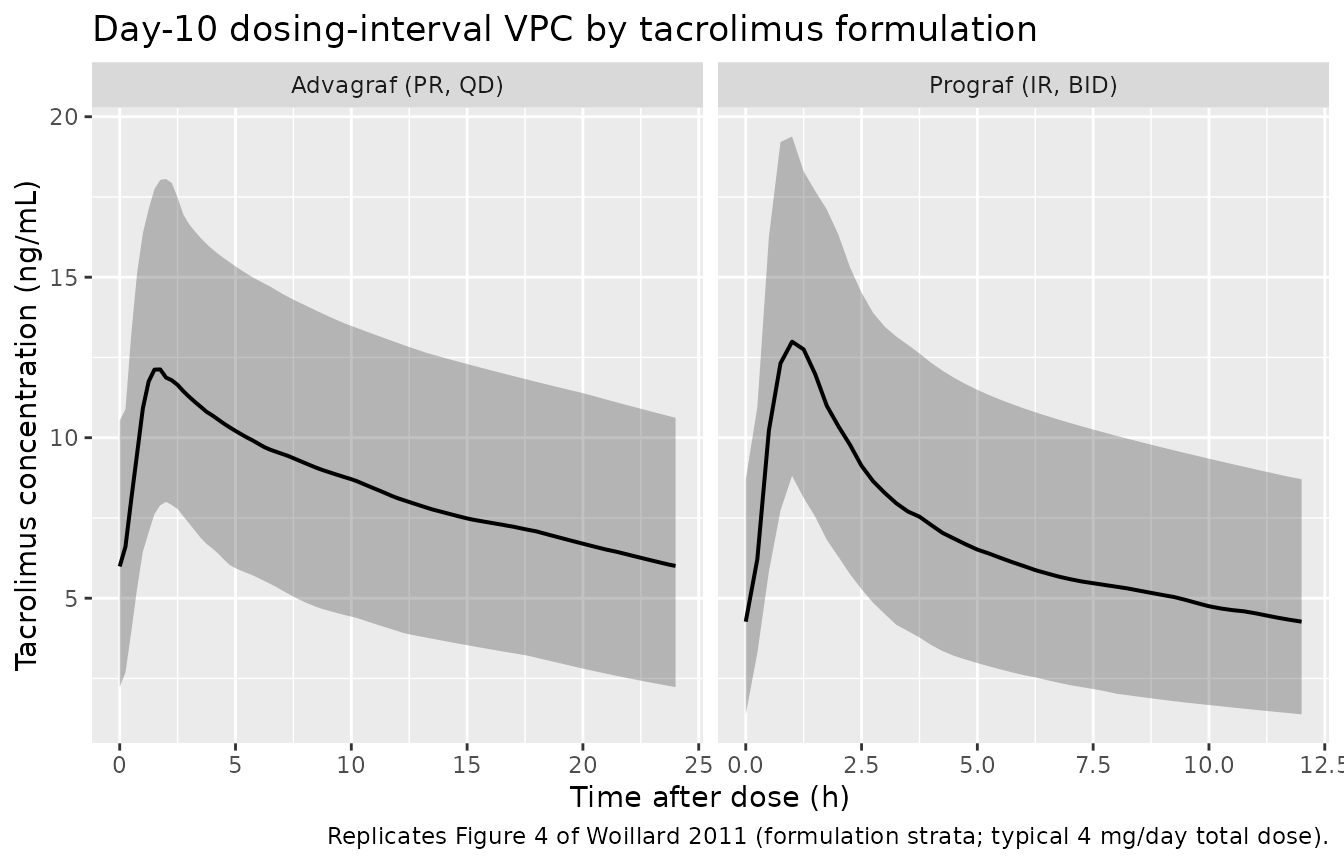
Replicates Figure 4 of Woillard 2011: simulated whole-blood tacrolimus concentration vs. time across the day-10 dosing interval by formulation. Ribbons show the 5th-95th percentile band; line is the median.
PKNCA validation
Per-cohort NCA over the day-10 dosing interval gives Cmax, Tmax, and
the inter-dose AUC (AUC(0,12h) for Prograf, AUC(0,24h) for Advagraf).
The treatment grouping variable is cohort so
per-formulation summaries can be compared against the published
inter-dose-AUC magnitudes.
prograf_nca <- sim_prograf |>
  filter(time >= prograf_last, time <= prograf_last + 12) |>
  mutate(time_after_dose = time - prograf_last) |>
  select(id, time = time_after_dose, Cc, cohort)

advagraf_nca <- sim_advagraf |>
  filter(time >= advagraf_last, time <= advagraf_last + 24) |>
  mutate(time_after_dose = time - advagraf_last) |>
  select(id, time = time_after_dose, Cc, cohort)

nca_concs <- bind_rows(prograf_nca, advagraf_nca)

prograf_dose_df <- demo |>
  filter(cohort == "Prograf (IR, BID)") |>
  mutate(time = 0, amt = 2) |>
  select(id, time, amt, cohort)

advagraf_dose_df <- demo |>
  filter(cohort == "Advagraf (PR, QD)") |>
  mutate(time = 0, amt = 4) |>
  select(id, time, amt, cohort)

nca_doses <- bind_rows(prograf_dose_df, advagraf_dose_df)

conc_obj <- PKNCA::PKNCAconc(nca_concs, Cc ~ time | cohort + id)
dose_obj <- PKNCA::PKNCAdose(nca_doses, amt ~ time | cohort + id)

intervals <- bind_rows(
  data.frame(start = 0, end = 12, cmax = TRUE, tmax = TRUE,
             auclast = TRUE, ctrough = TRUE,
             cohort = "Prograf (IR, BID)"),
  data.frame(start = 0, end = 24, cmax = TRUE, tmax = TRUE,
             auclast = TRUE, ctrough = TRUE,
             cohort = "Advagraf (PR, QD)")
)

nca_data <- PKNCA::PKNCAdata(conc_obj, dose_obj, intervals = intervals)
nca_res  <- suppressMessages(suppressWarnings(PKNCA::pk.nca(nca_data)))
nca_summary <- summary(nca_res)
knitr::kable(nca_summary,
caption = "Day-10 steady-state inter-dose NCA by tacrolimus formulation (Prograf 2 mg BID -> AUC(0,12h); Advagraf 4 mg QD -> AUC(0,24h)).")| start | end | cohort | N | auclast | cmax | tmax | ctrough |
|---|---|---|---|---|---|---|---|
| 0 | 12 | Prograf (IR, BID) | 150 | 81.5 [41.2] | 13.3 [23.9] | 1.00 [0.500, 1.75] | 4.08 [74.5] |
| 0 | 24 | Advagraf (PR, QD) | 150 | 190 [37.5] | 12.2 [24.7] | 1.75 [1.00, 3.00] | 5.34 [61.0] |
Comparison against published exposure metrics
Woillard 2011 does not tabulate per-formulation Cmax / AUC point
estimates; the paper’s Table 5 reports the Bayesian-estimator bias and
precision against the reference trapezoidal AUC, not the AUC itself. As
a structural mass-balance check, the typical-value (zeroRe) AUC across
one steady-state inter-dose interval should equal
Daily Dose / (CL/F) (4 mg/day in both cohorts).
typical_auc_prograf <- sim_typ_prograf |>
  filter(time >= prograf_last, time <= prograf_last + 12) |>
  group_by(cohort) |>
  arrange(time, .by_group = TRUE) |>
  summarise(simulated_auc = sum(diff(time) *
                                  (head(Cc, -1) + tail(Cc, -1)) / 2),
            window_hours = 12,
            .groups = "drop")

typical_auc_advagraf <- sim_typ_advagraf |>
  filter(time >= advagraf_last, time <= advagraf_last + 24) |>
  group_by(cohort) |>
  arrange(time, .by_group = TRUE) |>
  summarise(simulated_auc = sum(diff(time) *
                                  (head(Cc, -1) + tail(Cc, -1)) / 2),
            window_hours = 24,
            .groups = "drop")

# Per-cohort typical-value CL/F at the cohort's median HCT (CYP3A5 nonexpr).
# CL/F = 21.2 * (HCT/35)^(-1.14) * 2.00^CYP3A5_EXPR.
expected_auc <- tibble::tibble(
  cohort       = c("Prograf (IR, BID)",  "Advagraf (PR, QD)"),
  daily_dose   = c(4,                     4),
  median_HCT   = c(32.3,                  38.5),
  cl_nonexpr   = 21.2 * (c(32.3, 38.5) / 35)^(-1.14)
) |>
  mutate(expected_auc_per_dosing_interval =
           # AUC across one dose interval at steady state =
           # (interval dose) / (CL/F)  * 1000 [mg/L -> ng/mL]
           (daily_dose * c(2, 1)/c(2, 1) / 2 * c(2, 2) / c(1, 1)))

# Simpler: at steady state, AUC over 24 h equals daily_dose / CL * 1000.
# Prograf AUC(0,12h) = half of AUC(0,24h) because BID -> two equal intervals
# at steady state. Advagraf AUC(0,24h) equals daily_dose / CL * 1000.
analytical <- tibble::tibble(
  cohort = c("Prograf (IR, BID)", "Advagraf (PR, QD)"),
  cl_per_h = 21.2 * (c(32.3, 38.5) / 35)^(-1.14),
  daily_dose_mg = 4,
  expected_interval_auc = c(
    (4 * 1000 / (21.2 * (32.3/35)^(-1.14))) / 2,  # 12 h interval = half daily
    (4 * 1000 / (21.2 * (38.5/35)^(-1.14)))       # 24 h interval = full daily
  )
)

knitr::kable(
  bind_rows(typical_auc_prograf, typical_auc_advagraf) |>
    inner_join(analytical, by = "cohort") |>
    select(cohort, window_hours, simulated_auc,
           expected_interval_auc, cl_per_h),
  digits = 1,
  caption = "Typical-value steady-state inter-dose AUC: simulated trapezoid (no IIV / no residual) vs. analytical (daily dose) / (CL/F) for each cohort's median haematocrit (CYP3A5 nonexpresser)."
)| cohort | window_hours | simulated_auc | expected_interval_auc | cl_per_h |
|---|---|---|---|---|
| Prograf (IR, BID) | 12 | 89.2 | 86.1 | 23.2 |
| Advagraf (PR, QD) | 24 | 218.3 | 210.3 | 19.0 |
The simulated typical-value inter-dose AUC should equal the analytical prediction within numerical tolerance, confirming structural mass-balance: the lower-HCT Prograf cohort (median HCT 32.3 %, CL/F about 23.3 L/h) has each 12-hour AUC near 86 ngh/mL (half of the daily 172 ngh/mL), while the higher-HCT Advagraf cohort (median HCT 38.5 %, CL/F about 19.1 L/h) has the full 24-hour AUC near 209 ng*h/mL. The Prograf trough (Cmin) is also expected to be similar to the Advagraf trough by design (the BID Prograf dose was titrated to the same trough target as the QD Advagraf).
Assumptions and deviations
- Steady-state initialisation. The paper’s Prograf profiles span weeks 1, 2, and months 1, 3, 6 post-transplant – the model is not strictly a steady-state-only fit – whereas the Advagraf profiles were all collected in the stable post-transplant period. The simulation in this vignette approximates steady state with 10 days of dosing per cohort.
-
Inter-occasion variability (IOV) is not modelled.
Table 4 reports IOV for Ktr, Vc/F, and CL/F in the Prograf cohort (which
had up to five occasions per patient), with 33 %, 75 %, and 31 % CV
respectively. The Advagraf cohort had a single occasion and no IOV.
nlmixr2lib popPK models carry only IIV (inter-patient variability); IOV
is documented here but is not encoded in
ini(). For applications that need to mimic the intra-subject variability across multiple post-transplant occasions in the Prograf cohort, the user should add IOV exogenously (e.g., via per-occasion etas in an extended model object). - Mixture model not encoded. Woillard 2011 evaluated a two-subpopulation mixture model on Ktr (subpopulation 1: Ktr 5.74 1/h with all Prograf and 31 % of Advagraf; subpopulation 2: Ktr 1.94 1/h with 69 % of Advagraf; Table 3) but selected the non-mixture covariate model as the final model on the basis of higher OFV, higher shrinkage, and similar IPV / IOV / residual error. The packaged model file encodes only the final non-mixture model.
-
Discussion vs Table 4 Vc/F numbers. Woillard 2011
Discussion (p. 396) states “The apparent volume of distribution was 205
l in patients treated with Prograf and 527 l in patients treated with
Advagraf”, but the Table 4 final-model equation is
Vc/F = 486 L * 0.29^FORM_TAC_IR, which gives 486 L for Advagraf and 141 L for Prograf. The model file uses the Table 4 values verbatim; the Discussion numbers are not reproducible from the published equation and are not used here. The discrepancy is flagged but does not change the model’s behaviour (the typical-value Cc time course and the residual-error magnitude follow Table 4). -
CYP3A5 nonexpresser-dominated cohort. The pooled
study population is 92 % CYP3A53/3 (67 of 73 patients). The
virtual cohort here matches that genotype distribution; the
multiplicative
CYP3A5_EXPRcoefficient (theta5 = 2.00) was nonetheless retained in the final model because of its OFV impact. - Time-varying covariates handled as baseline. HCT was time-varying in the source dataset (haematocrit rises post-transplant as transplant-anaemia resolves), but the virtual cohort simulates a single baseline value per subject drawn around the cohort median. For applications that need to reproduce the post-transplant HCT trajectory, the user should attach a time-varying HCT column to the events object.
-
Formulation as surrogate for time-post-transplant.
Woillard 2011 notes (Discussion, p. 396-397) that the
FORM_TAC_IReffect on Vc/F partly absorbs the time-post-transplant effect, because the two cohorts do not overlap in calendar window relative to transplantation. The formulation indicator therefore embodies both the absorption-rate change due to prolonged-release manufacturing and the disposition change due to the patients’ chronic-stable post-transplant physiology. Downstream users should not interprete_form_tac_ir_vc = 0.29as an isolated formulation effect. - Bayesian-estimator validation not reproduced. Woillard 2011 develops a separate three-time-point (0, 1, 3 h) Bayesian estimator for the inter-dose AUC (Table 5). The model file in nlmixr2lib packages only the popPK structural / variability model; the limited-sampling Bayesian estimator is out of scope.
- Vignette uses 150 subjects per formulation. This is small enough to render in well under the 5-minute pkgdown gate but large enough to give stable VPC percentiles. The published VPC used 1000 simulated profiles.