Nemonoxacin (Chen 2023)
Source:vignettes/articles/Chen_2023_nemonoxacin.Rmd
Chen_2023_nemonoxacin.RmdModel and source
- Citation: Chen Y, Wu X, Tsai C, Chang L, Yu J, Cao G, Guo B, Shi Y, Zhu D, Hu F, Yuan J, Liu Y, Zhao X, Zhang Y, Wu J, Zhang J (2023). Integrative population pharmacokinetic/pharmacodynamic analysis of nemonoxacin capsule in Chinese patients with community-acquired pneumonia. Frontiers in Pharmacology 14:912962. doi:10.3389/fphar.2023.912962.
- Description: Two-compartment population PK model for oral nemonoxacin capsules in Chinese adults, pooled across phase I to III trials (Chen 2023; n = 161 subjects / 195 cases; 2007 plasma concentrations). First-order absorption with a lag time and estimated relative bioavailability. Clearance is an additive linear function of Cockcroft-Gault creatinine clearance (10.3 L/h intercept + 0.026 L/h per mL/min), and allometric body-weight scaling is fixed at 0.75 on CL / Q and 1 on Vc / Vp with a 70 kg reference. Covariate effects: female sex lowers Vc by 11%; community-acquired pneumonia raises Vp by 23%; food slows absorption (ka x 0.44), lengthens the lag time (T_lag x 1.6), and lowers bioavailability (F x 0.88). Inter-occasion variability on CL distinguishes the single-dose occasion from steady state (72 h after the first of multiple doses). The paper’s companion PK/PD analysis is an exposure-response logistic regression on AUC0-24/MIC, Cmax/MIC and %T > MIC; its regression coefficients are not reported, so only the population PK layer is encoded here (the published PK/PD targets are reproduced in the validation vignette).
- Article: Front Pharmacol 14:912962
Nemonoxacin is a non-fluorinated quinolone (TG-873870) developed for community-acquired pneumonia (CAP). Chen 2023 pooled the oral-capsule PK data from three Chinese trials into a single population PK model and then used it to derive PK/PD targets and Monte Carlo target-attainment estimates. This vignette reproduces the population PK layer.
Population
The analysis pooled 161 subjects (195 cases, 2027 plasma
concentrations, of which 2007 were retained) across three trials of oral
nemonoxacin capsule: the phase I trial TG-873870-C-1 in
healthy subjects, the phase II CAP trial TG-873870-C-3, and
the phase III CAP trial versus levofloxacin TG-873870-C-4.
The cohort comprised 125 CAP patients and 36 healthy subjects, 111 male
and 84 female, aged 18-70 years (mean 34.0 +/- 14.4, median 27.5),
weighing 42-90 kg (mean 61.0 +/- 9.0, median 60), with Cockcroft-Gault
creatinine clearance 50.7-200.7 mL/min (mean 114.4 +/- 29.2, median
116.2). All subjects were Chinese. 91 of 195 cases were dosed in the fed
state (food within 2 h before or 30 min after the dose). Baseline
characteristics are Chen 2023 Table 1.
Two exclusions matter for interpreting the model. Subjects aged 75 years or older and subjects with moderate or severe renal impairment were excluded from all three trials, so the paper’s renal-impairment predictions (and any simulation below CLcr ~50 mL/min) are extrapolations outside the observed covariate range – a limitation the authors state explicitly in the Discussion.
The same information is available programmatically via the model’s
population metadata
(readModelDb("Chen_2023_nemonoxacin")()$population).
Source trace
Every ini() entry in
inst/modeldb/specificDrugs/Chen_2023_nemonoxacin.R carries
an in-file comment naming its origin. The table below collects them for
review. Table 2 values are the “Estimate based on original dataset”
column; the covariate model is Chen 2023 Eq. 8.
| Equation / parameter | Value | Source location |
|---|---|---|
| Structural model: 2-compartment, first-order absorption with lag | n/a | Results “PPK model”: “The base PPK model of nemonoxacin was a two-compartment model, where the absorption was a first-order process with a Tlag.” |
Exponential IIV
Para_ind = Para_pop * exp(eta + kappa)
|
n/a | Eq. 1 |
Mixed residual error Y = Ypred * (1 + eps1) + eps2
|
n/a | Eq. 2 |
| Full covariate model | n/a | Eq. 8 |
lcl (CL intercept at CLcr = 0, 70 kg) |
10.3 L/h | Table 2 row “CL”; Eq. 8 |
e_crcl_cl (additive CLcr slope on CL) |
0.026 L/h per mL/min | Table 2 row “CLcr (CL)”; Eq. 8 |
lvc (Vc, 70 kg, male) |
103 L | Table 2 row “V2”; Eq. 8 |
lq (Q, 70 kg) |
2.0 L/h | Table 2 row “Q”; Eq. 8 |
lvp (Vp, 70 kg, CAP patient) |
28 x 1.23 = 34.4 L | Table 2 row “V3” (28 L, healthy) x Eq. 8 DisStat factor |
lka (ka, fasted) |
2.2 1/h | Table 2 row “KA”; Eq. 8 |
ltlag (T_lag, fasted) |
0.19 h | Table 2 row “TLAG”; Eq. 8 |
lfdepot (F1 anchor, fasted) |
1, fixed | Eq. 8 “F1 = 1 x 0.88^Food”; no typical-value row in Table 2 |
e_wt_cl_q (allometric exponent on CL, Q) |
0.75, fixed | Methods “Fixed effect model”, priori-information paragraph |
e_wt_vc_vp (allometric exponent on Vc, Vp) |
1, fixed | Methods “Fixed effect model”, priori-information paragraph |
e_sexf_vc (female factor on Vc) |
0.89 | Table 2 row “SEX (V2)”; Eq. 8 0.89^Sex
|
e_dis_healthy_vp (healthy factor on Vp) |
1 / 1.23 = 0.813 | Eq. 8 1.23^DisStat, re-expressed onto
DIS_HEALTHY = 1 - DisStat
|
e_fed_ka (fed factor on ka) |
0.44 | Table 2 row “Food (Ka)”; Eq. 8 0.44^Food
|
e_fed_tlag (fed factor on T_lag) |
1.6 | Table 2 row “Food (TLAG)”; Eq. 8 1.6^Food
|
e_fed_fdepot (fed factor on F1) |
0.88 | Table 2 row “Food(F)”; Eq. 8 0.88^Food
|
etalcl (IIV CL) |
0.0013 | Table 2 row “omega^2 CL”; SD 3.6% per Results |
etalvc (IIV Vc) |
0.0034 | Table 2 row “omega^2 V2”; SD 5.7% per Results |
etalvp (IIV Vp) |
0.0080 | Table 2 row “omega^2 V3”; SD 8.8% per Results |
etalka (IIV ka) |
0.64 | Table 2 row “omega^2 KA”; SD 81% per Results |
etaltlag (IIV T_lag) |
0.71 | Table 2 row “omega^2 TLAG”; SD 83% per Results |
etalfdepot (IIV F) |
0.035 | Table 2 row “omega^2 F”; SD 19% per Results |
etaiov_cl_1, etaiov_cl_2 (IOV CL) |
0.017 | Table 2 row “pi^2 CL”; IOV SD 13% per Results; occasion 2 fixed SAME |
propSd |
sqrt(0.032) = 0.179 | Table 2 row “sigma^2 prop” |
addSd |
sqrt(0.34e-4) = 0.00583 mg/L | Table 2 row “sigma^2 add” (unit column 10^-4) |
| PK/PD targets (validation only) | see below | Table 3 |
| PK/PD cutoff values (validation only) | see below | Table 4 |
Virtual cohort
Original observed data are not publicly available. The cohort below
is a virtual CAP population whose covariate distributions approximate
Chen 2023 Table 1 (CAP-patient column): body weight 61.9 +/- 9.8 kg
truncated to the observed 42-90 kg, Cockcroft-Gault CLcr 103.8 +/- 27.9
mL/min truncated to the observed 50.7-187.5 mL/min, and 48 of 125
female. All records are fasted (FED = 0), so the simulation
is referenced to the paper’s structural fasted state.
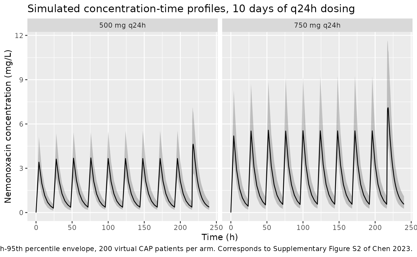
Two arms of 200 subjects each cover the regimens the paper carried into Monte Carlo simulation: 500 mg and 750 mg once daily for 10 days.
set.seed(20230228)

n_per_arm <- 200L
tau <- 24      # dosing interval (h)
n_doses <- 10L # 10 days of q24h dosing

# Inverse-CDF truncated normal, so the truncation does not pile mass on the
# bounds the way clamping would.
rtnorm <- function(n, mean, sd, lo, hi) {
  u <- runif(n, stats::pnorm(lo, mean, sd), stats::pnorm(hi, mean, sd))
  stats::qnorm(u, mean, sd)
}

dose_times <- seq(0, (n_doses - 1L) * tau, by = tau)

# Fine grid over the final dosing interval, where the steady-state NCA is taken.
# 15-minute resolution is needed to resolve Tmax (about 1.6 h fasted).
obs_times_ss <- seq((n_doses - 1L) * tau, n_doses * tau, by = 0.25)

# Full grid: the steady-state interval plus a coarse grid over the accumulation
# phase for the concentration-time figure. Kept deliberately coarse -- the
# figure only needs to show the approach to steady state, and observation rows
# are the main driver of render time.
obs_times <- sort(unique(c(seq(0, (n_doses - 1L) * tau, by = 4), obs_times_ss)))

make_cohort <- function(n, dose_mg, treatment, id_offset = 0L) {
  subj <- tibble(
    id           = id_offset + seq_len(n),
    WT           = rtnorm(n, 61.9, 9.8, 42, 90),
    CRCL         = rtnorm(n, 103.8, 27.9, 50.7, 187.5),
    SEXF         = rbinom(n, 1L, 48 / 125),
    DIS_HEALTHY  = 0L,   # CAP patients
    FED          = 0L,   # fasted
    treatment    = treatment
  )

  doses <- subj |>
    tidyr::crossing(time = dose_times) |>
    mutate(amt = dose_mg, evid = 1L, cmt = "depot")

  obs <- subj |>
    tidyr::crossing(time = obs_times) |>
    mutate(amt = NA_real_, evid = 0L, cmt = "central")

  bind_rows(doses, obs) |>
    # OCC = 1 is the single-dose occasion; OCC = 2 is steady state, which
    # Chen 2023 defines as 72 h after the first of multiple doses.
    mutate(OCC = if_else(time < 72, 1L, 2L)) |>
    arrange(id, time, desc(evid)) |>
    as.data.frame()
}

events <- bind_rows(
  make_cohort(n_per_arm, 500, "500 mg q24h", id_offset = 0L),
  make_cohort(n_per_arm, 750, "750 mg q24h", id_offset = n_per_arm)
)

stopifnot(!anyDuplicated(events[, c("id", "time", "evid")]))
Simulation
mod <- readModelDb("Chen_2023_nemonoxacin")

sim <- rxode2::rxSolve(mod, events = events, keep = c("treatment")) |>
  as.data.frame()
#> ℹ parameter labels from comments will be replaced by 'label()'
#> Warning: some etas defaulted to non-mu referenced, possible parsing error: etaiov_cl_1, etaiov_cl_2
#> as a work-around try putting the mu-referenced expression on a simple line
Replicate published figures
Chen 2023’s own PK figures are goodness-of-fit plots (Figure 1) and a visual predictive check (Supplementary Figure S2) built on the observed data, neither of which can be redrawn without the trial dataset. The panel below is the corresponding forward simulation: median and 5th-95th percentile concentration envelopes over 10 days of once-daily dosing, which is the quantity the VPC compares against.
# Corresponds to Supplementary Figure S2 of Chen 2023 (VPC for the final PPK
# model); shown here as the model's forward-simulated prediction interval.
sim |>
  filter(!is.na(Cc)) |>
  group_by(treatment, time) |>
  summarise(
    Q05 = quantile(Cc, 0.05),
    Q50 = quantile(Cc, 0.50),
    Q95 = quantile(Cc, 0.95),
    .groups = "drop"
  ) |>
  ggplot(aes(time, Q50)) +
  geom_ribbon(aes(ymin = Q05, ymax = Q95), alpha = 0.25) +
  geom_line() +
  facet_wrap(~treatment) +
  labs(
    x = "Time (h)", y = "Nemonoxacin concentration (mg/L)",
    title = "Simulated concentration-time profiles, 10 days of q24h dosing",
    caption = paste(
      "Median with 5th-95th percentile envelope, 200 virtual CAP patients per",
      "arm. Corresponds to Supplementary Figure S2 of Chen 2023."
    )
  )
PKNCA validation
Steady-state NCA is taken over the final dosing interval (216-240 h), matching the paper’s “AUC0-24 and Cmax of nemonoxacin at steady state” (Methods, “PPK simulation”).
start_ss <- max(dose_times)
end_ss   <- start_ss + tau

sim_nca <- sim |>
  filter(!is.na(Cc)) |>
  select(id, time, Cc, treatment)

# Guarantee a time-zero record per subject; for extravascular dosing a
# pre-dose concentration of 0 is the correct anchor for PKNCA.
sim_nca <- bind_rows(
  sim_nca,
  sim_nca |> distinct(id, treatment) |> mutate(time = 0, Cc = 0)
) |>
  distinct(id, treatment, time, .keep_all = TRUE) |>
  arrange(id, treatment, time)

conc_obj <- PKNCA::PKNCAconc(
  sim_nca, Cc ~ time | treatment + id,
  concu = "mg/L", timeu = "h"
)

dose_df <- events |>
  filter(evid == 1L) |>
  select(id, time, amt, treatment)

dose_obj <- PKNCA::PKNCAdose(dose_df, amt ~ time | treatment + id)

intervals <- data.frame(
  start     = start_ss,
  end       = end_ss,
  cmax      = TRUE,
  tmax      = TRUE,
  cmin      = TRUE,
  auclast   = TRUE,
  half.life = TRUE
)

nca_res <- PKNCA::pk.nca(
  PKNCA::PKNCAdata(conc_obj, dose_obj, intervals = intervals)
)
Comparison against published NCA
Chen 2023’s Results section reports the model-predicted steady-state exposures directly: “nemonoxacin AUC0-24 was 42.0 and 65.5 mg h/L, respectively after administration of 500 mg or 750 mg … The predicted Cmax was 5.00 and 7.50 mg/L following dose of 500 or 750 mg”. Those Bayesian model predictions are the reference below, because reproducing them is the direct test of whether this re-implementation of Eq. 8 matches the published model.
For context, the corresponding observed values in CAP patients were AUC0-24 46.9 (500 mg) and 62.5 mg h/L (750 mg), and Cmax 5.42 (500 mg) and 8.49 mg/L (750 mg).
published <- tibble::tribble(
  ~treatment,     ~cmax, ~auclast,
  "500 mg q24h",  5.00,  42.0,
  "750 mg q24h",  7.50,  65.5
)

cmp <- nlmixr2lib::ncaComparisonTable(
  simulated = nca_res,
  reference = published,
  by        = "treatment",
  units     = c(cmax = "mg/L", auclast = "mg*h/L"),
  tolerance_pct = 20
)

knitr::kable(
  cmp,
  caption = paste(
    "Simulated steady-state NCA (median of 200 virtual CAP patients per arm,",
    "final 24 h dosing interval) vs the Bayesian model predictions reported in",
    "Chen 2023 Results. * differs from the reference by >20%."
  ),
  align = c("l", "l", "r", "r", "r")
)| NCA parameter | treatment | Reference | Simulated | % diff |
|---|---|---|---|---|
| Cmax (mg/L) | 500 mg q24h | 5 | 4.79 | -4.1% |
| Cmax (mg/L) | 750 mg q24h | 7.5 | 7.52 | +0.3% |
| AUClast (mg*h/L) | 500 mg q24h | 42 | 41.6 | -1.0% |
| AUClast (mg*h/L) | 750 mg q24h | 65.5 | 63.4 | -3.1% |
attr(cmp, "footnote")
#> NULL
The full simulated distribution, for reference:
as.data.frame(nca_res) |>
  filter(PPTESTCD %in% c("cmax", "tmax", "cmin", "auclast", "half.life")) |>
  group_by(treatment, PPTESTCD) |>
  summarise(
    Median = median(PPORRES, na.rm = TRUE),
    P05    = quantile(PPORRES, 0.05, na.rm = TRUE),
    P95    = quantile(PPORRES, 0.95, na.rm = TRUE),
    .groups = "drop"
  ) |>
  rename(
    "Treatment"     = treatment,
    "NCA parameter" = PPTESTCD
  ) |>
  knitr::kable(
    digits = 3,
    caption = paste(
      "Simulated steady-state NCA distribution over the final dosing interval.",
      "Cmax and Cmin in mg/L, tmax and half.life in h, auclast in mg*h/L."
    )
)| Treatment | NCA parameter | Median | P05 | P95 |
|---|---|---|---|---|
| 500 mg q24h | auclast | 41.561 | 27.003 | 64.996 |
| 500 mg q24h | cmax | 4.793 | 2.926 | 7.550 |
| 500 mg q24h | cmin | 0.364 | 0.187 | 0.707 |
| 500 mg q24h | half.life | 8.142 | 7.148 | 9.379 |
| 500 mg q24h | tmax | 1.625 | 0.750 | 3.500 |
| 750 mg q24h | auclast | 63.444 | 41.248 | 105.038 |
| 750 mg q24h | cmax | 7.523 | 4.853 | 12.264 |
| 750 mg q24h | cmin | 0.558 | 0.261 | 1.065 |
| 750 mg q24h | half.life | 8.138 | 7.268 | 9.193 |
| 750 mg q24h | tmax | 1.500 | 0.750 | 3.250 |
Covariate effects on steady-state exposure
Chen 2023 quantifies each retained covariate by simulating the model and recomputing steady-state NCA (Results, “Effect of covariates on PK”, reported in Supplementary Figures S3-S10). Those percentage changes are a sharper test of the covariate model than any single exposure value, because each one isolates a single covariate.
They are checked here in two ways. Clearance, volume, and steady-state AUC are closed-form functions of Eq. 8, so they are evaluated exactly from the coefficients stored in the packaged model – no simulation, and therefore no dependence on the solver. Cmax, Tmax, and Cmin are not closed-form, so they are taken from paired stochastic cohorts: the same virtual subjects are simulated twice with a single covariate flipped, which removes between-cohort sampling noise from the comparison.
Closed-form covariate algebra
The coefficients are read back out of the packaged model rather than
retyped, so this block tests the values actually stored in
inst/modeldb/specificDrugs/Chen_2023_nemonoxacin.R.
ui <- readModelDb("Chen_2023_nemonoxacin")()
#> Warning: some etas defaulted to non-mu referenced, possible parsing error: etaiov_cl_1, etaiov_cl_2
#> as a work-around try putting the mu-referenced expression on a simple line
th <- setNames(ui$iniDf$est, ui$iniDf$name)

# Eq. 8, typical values (all etas at zero).
cl_of  <- function(WT, CRCL) {
  (exp(th[["lcl"]]) + th[["e_crcl_cl"]] * CRCL) * (WT / 70)^th[["e_wt_cl_q"]]
}
vc_of  <- function(WT, SEXF) {
  exp(th[["lvc"]]) * (WT / 70)^th[["e_wt_vc_vp"]] * th[["e_sexf_vc"]]^SEXF
}
vp_of  <- function(WT, DIS_HEALTHY) {
  exp(th[["lvp"]]) * (WT / 70)^th[["e_wt_vc_vp"]] *
    th[["e_dis_healthy_vp"]]^DIS_HEALTHY
}
f_of   <- function(FED) exp(th[["lfdepot"]]) * th[["e_fed_fdepot"]]^FED

# Apparent (oral) quantities, which is what the paper reports. At steady state
# with a linear model, AUC0-tau = Dose * F / CL exactly.
metrics_of <- function(WT, CRCL, SEXF, DIS_HEALTHY, FED, dose = 500) {
  f <- f_of(FED)
  c(
    clf     = cl_of(WT, CRCL) / f,
    vssf    = (vc_of(WT, SEXF) + vp_of(WT, DIS_HEALTHY)) / f,
    auclast = dose * f / cl_of(WT, CRCL)
  )
}

# Sanity check that the stored coefficients are the published ones.
stopifnot(
  abs(exp(th[["lcl"]])          - 10.3)      < 1e-8,
  abs(th[["e_crcl_cl"]]         - 0.026)     < 1e-12,
  abs(exp(th[["lvc"]])          - 103)       < 1e-8,
  abs(exp(th[["lvp"]])          - 28 * 1.23) < 1e-8,
  abs(th[["e_sexf_vc"]]         - 0.89)      < 1e-12,
  abs(th[["e_dis_healthy_vp"]]  - 1 / 1.23)  < 1e-12,
  abs(th[["e_fed_fdepot"]]      - 0.88)      < 1e-12
)
# Each row: the paper's stated percentage change, and the same change evaluated
# from Eq. 8. Covariates not under test are held at the cohort-typical CAP
# values (61.9 kg, CLcr 103.8 mL/min, male, fasted).
closed_form_claims <- tibble::tribble(
  ~comparison,      ~metric,   ~paper_pct, ~ref,                              ~test,                             ~source,
  "BW 80 vs 60 kg", "clf",     25,  list(60, 103.8, 0, 0, 0),   list(80, 103.8, 0, 0, 0),   "Results: 'CLss/F and Vss/F increased by 25% and 29%'",
  "BW 80 vs 60 kg", "vssf",    29,  list(60, 103.8, 0, 0, 0),   list(80, 103.8, 0, 0, 0),   "Results: 'CLss/F and Vss/F increased by 25% and 29%'",
  "BW 80 vs 60 kg", "auclast", -19, list(60, 103.8, 0, 0, 0),   list(80, 103.8, 0, 0, 0),   "Results: 'Cmax and AUC0-24,ss reduced by 24% and 19%'",
  "CLcr 30 vs 150", "auclast", 28,  list(61.9, 150, 0, 0, 0),   list(61.9, 30, 0, 0, 0),    "Abstract: 'AUC0-24,ss and T1/2 increased by 28% and 24%'",
  "CLcr 75 vs 200", "clf",     -22, list(61.9, 200, 0, 0, 0),   list(61.9, 75, 0, 0, 0),    "Results: 'Vss/F and CLss/F of nemonoxacin reduced by 8% and 22%'",
  "CLcr 75 vs 200", "auclast", 28,  list(61.9, 200, 0, 0, 0),   list(61.9, 75, 0, 0, 0),    "Results: mild renal insufficiency, 'AUC0-24,ss increased by 28%'",
  "CLcr 15 vs 200", "auclast", 47,  list(61.9, 200, 0, 0, 0),   list(61.9, 15, 0, 0, 0),    "Results: renal failure, 'AUC0-24,ss increased by 47%'",
  "Fed vs fasted",  "vssf",    24,  list(61.9, 103.8, 0, 0, 0), list(61.9, 103.8, 0, 0, 1), "Results: 'Vss/F increased by 24%'"
)

closed_form_claims |>
  rowwise() |>
  mutate(
    reference = metrics_of(ref[[1]],  ref[[2]],  ref[[3]],  ref[[4]],  ref[[5]])[[metric]],
    predicted = metrics_of(test[[1]], test[[2]], test[[3]], test[[4]], test[[5]])[[metric]]
  ) |>
  ungroup() |>
  mutate(
    model_pct = 100 * (predicted - reference) / reference,
    diff      = model_pct - paper_pct,
    flag      = if_else(abs(diff) > 5, "*", "")
  ) |>
  select(comparison, metric, paper_pct, model_pct, diff, flag, source) |>
  rename(
    "Comparison"      = comparison,
    "Metric"          = metric,
    "Chen 2023 (%)"   = paper_pct,
    "Model (%)"       = model_pct,
    "Difference (pp)" = diff,
    "Flag"            = flag,
    "Source"          = source
  ) |>
  knitr::kable(
    digits = 1,
    caption = paste(
      "Covariate effects evaluated in closed form from the packaged model's",
      "Eq. 8 coefficients, against the percentage changes reported by",
      "Chen 2023. * marks a discrepancy larger than 5 percentage points."
    )
)| Comparison | Metric | Chen 2023 (%) | Model (%) | Difference (pp) | Flag | Source |
|---|---|---|---|---|---|---|
| BW 80 vs 60 kg | clf | 25 | 24.1 | -0.9 | Results: ‘CLss/F and Vss/F increased by 25% and 29%’ | |
| BW 80 vs 60 kg | vssf | 29 | 33.3 | 4.3 | Results: ‘CLss/F and Vss/F increased by 25% and 29%’ | |
| BW 80 vs 60 kg | auclast | -19 | -19.4 | -0.4 | Results: ‘Cmax and AUC0-24,ss reduced by 24% and 19%’ | |
| CLcr 30 vs 150 | auclast | 28 | 28.2 | 0.2 | Abstract: ‘AUC0-24,ss and T1/2 increased by 28% and 24%’ | |
| CLcr 75 vs 200 | clf | -22 | -21.0 | 1.0 | Results: ‘Vss/F and CLss/F of nemonoxacin reduced by 8% and 22%’ | |
| CLcr 75 vs 200 | auclast | 28 | 26.5 | -1.5 | Results: mild renal insufficiency, ‘AUC0-24,ss increased by 28%’ | |
| CLcr 15 vs 200 | auclast | 47 | 45.0 | -2.0 | Results: renal failure, ‘AUC0-24,ss increased by 47%’ | |
| Fed vs fasted | vssf | 24 | 13.6 | -10.4 | * | Results: ‘Vss/F increased by 24%’ |
Paired stochastic cohorts for Cmax, Tmax, and Cmin
Cmax, Tmax, and Cmin depend on the whole concentration-time curve rather than on a single parameter, so they are read from simulation. Each comparison below reuses one base cohort of 60 virtual CAP patients (fasted, male, so that the food and sex covariates have somewhere to move to) and re-simulates the same subjects with one covariate flipped. Because the comparison is within-subject, 60 subjects per arm is ample; only the final dosing interval is observed, since that is the only window the NCA uses.
set.seed(20230301)

n_paired <- 60L

base_subj <- tibble(
  id   = seq_len(n_paired),
  WT   = rtnorm(n_paired, 61.9, 9.8, 42, 90),
  CRCL = rtnorm(n_paired, 103.8, 27.9, 50.7, 187.5)
)

# `arm` names the covariate state; `flip` is applied to the shared base cohort.
paired_arms <- tibble::tribble(
  ~arm,       ~SEXF, ~DIS_HEALTHY, ~FED,
  "base",     0L,    0L,           0L,
  "fed",      0L,    0L,           1L,
  "female",   1L,    0L,           0L,
  "healthy",  0L,    1L,           0L
)

make_paired <- function(i) {
  a <- paired_arms[i, ]
  subj <- base_subj |>
    mutate(
      # Offset ids so the arms stay distinct subjects within one solve.
      id          = id + (i - 1L) * n_paired,
      SEXF        = a$SEXF,
      DIS_HEALTHY = a$DIS_HEALTHY,
      FED         = a$FED,
      arm         = a$arm,
      pair        = row_number()
    )
  bind_rows(
    subj |> tidyr::crossing(time = dose_times) |>
      mutate(amt = 500, evid = 1L, cmt = "depot"),
    subj |> tidyr::crossing(time = obs_times_ss) |>
      mutate(amt = NA_real_, evid = 0L, cmt = "central")
  ) |>
    mutate(OCC = if_else(time < 72, 1L, 2L))
}

paired_events <- bind_rows(lapply(seq_len(nrow(paired_arms)), make_paired)) |>
  arrange(id, time, desc(evid)) |>
  as.data.frame()

paired_sim <- rxode2::rxSolve(
  mod, events = paired_events, keep = c("arm", "pair")
) |>
  as.data.frame()
paired_conc <- paired_sim |>
  filter(!is.na(Cc)) |>
  select(arm, pair, time, Cc)

paired_conc <- bind_rows(
  paired_conc,
  paired_conc |> distinct(arm, pair) |> mutate(time = 0, Cc = 0)
) |>
  distinct(arm, pair, time, .keep_all = TRUE) |>
  arrange(arm, pair, time)

paired_dose <- paired_events |>
  filter(evid == 1L) |>
  select(arm, pair, time, amt)

paired_nca <- PKNCA::pk.nca(PKNCA::PKNCAdata(
  PKNCA::PKNCAconc(paired_conc, Cc ~ time | arm + pair),
  PKNCA::PKNCAdose(paired_dose, amt ~ time | arm + pair),
  intervals = data.frame(
    start = start_ss, end = end_ss,
    cmax = TRUE, tmax = TRUE, cmin = TRUE
  )
))

# Per-subject ratio against that subject's own "base" record, then the median
# ratio. Pairing within subject removes cohort-to-cohort sampling noise.
paired_wide <- as.data.frame(paired_nca) |>
  select(arm, pair, PPTESTCD, PPORRES) |>
  tidyr::pivot_wider(names_from = arm, values_from = PPORRES)

paired_pct <- paired_wide |>
  tidyr::pivot_longer(
    c(fed, female, healthy), names_to = "arm", values_to = "value"
  ) |>
  mutate(ratio = value / base) |>
  group_by(arm, PPTESTCD) |>
  summarise(median_pct = 100 * (median(ratio) - 1), .groups = "drop")
# The paper's CAP-vs-healthy contrast runs the other way round (healthy is its
# reference), so the "healthy" arm's ratio is inverted to match.
paired_claims <- tibble::tribble(
  ~comparison,      ~arm,      ~PPTESTCD, ~paper_pct, ~invert, ~source,
  "Fed vs fasted",  "fed",     "tmax",    65,         FALSE,   "Results: 'Tmax increased by 1.2 h (65%)'",
  "Fed vs fasted",  "fed",     "cmax",    -23,        FALSE,   "Results: 'Cmax reduced by 23%'",
  "Female vs male", "female",  "cmin",    -13,        FALSE,   "Results: 'Cmin,ss reduced by 13% in female subjects'",
  "CAP vs healthy", "healthy", "cmin",    19,         TRUE,    "Results: 'Cmin,ss increased by 19% in CAP patients'",
  "CAP vs healthy", "healthy", "tmax",    11,         TRUE,    "Results: 'Tmax increased by 11%'"
)

paired_claims |>
  left_join(paired_pct, by = c("arm", "PPTESTCD")) |>
  mutate(
    sim_pct = if_else(
      invert, 100 * (1 / (1 + median_pct / 100) - 1), median_pct
    ),
    diff = sim_pct - paper_pct,
    flag = if_else(abs(diff) > 10, "*", "")
  ) |>
  select(comparison, PPTESTCD, paper_pct, sim_pct, diff, flag, source) |>
  rename(
    "Comparison"      = comparison,
    "Metric"          = PPTESTCD,
    "Chen 2023 (%)"   = paper_pct,
    "Simulated (%)"   = sim_pct,
    "Difference (pp)" = diff,
    "Flag"            = flag,
    "Source"          = source
  ) |>
  knitr::kable(
    digits = 1,
    caption = paste(
      "Cmax, Tmax, and Cmin covariate effects from paired stochastic cohorts",
      "(60 virtual CAP patients, each simulated in both covariate states);",
      "median of the per-subject ratio. * marks a discrepancy larger than 10",
      "percentage points."
    )
)| Comparison | Metric | Chen 2023 (%) | Simulated (%) | Difference (pp) | Flag | Source |
|---|---|---|---|---|---|---|
| Fed vs fasted | tmax | 65 | 66.7 | 1.7 | Results: ‘Tmax increased by 1.2 h (65%)’ | |
| Fed vs fasted | cmax | -23 | -28.2 | -5.2 | Results: ‘Cmax reduced by 23%’ | |
| Female vs male | cmin | -13 | -7.7 | 5.3 | Results: ‘Cmin,ss reduced by 13% in female subjects’ | |
| CAP vs healthy | cmin | 19 | -0.2 | -19.2 | * | Results: ‘Cmin,ss increased by 19% in CAP patients’ |
| CAP vs healthy | tmax | 11 | 20.7 | 9.7 | Results: ‘Tmax increased by 11%’ |
Reading the two tables
The closed-form comparisons reproduce the paper closely: every
clearance- and AUC-driven row agrees to within 2 percentage points. That
is the expected result and the main point of the check, because
steady-state AUC is Dose x F / CL exactly, so the
body-weight and creatinine-clearance comparisons reduce to ratios of
(10.3 + 0.026 x CLcr) x (BW/70)^0.75. Agreement this tight
confirms that Eq. 8 is transcribed correctly, including the additive
rather than multiplicative form of the CLcr term – the single most
easily mis-encoded feature of this model.
Two rows deserve comment.
Vss/F under food (-10.4 pp). The model’s apparent
Vss/F is (Vc + Vp) / F, which food changes only through the
12% reduction in F, i.e. +13.6%. The paper’s +24% is an NCA-derived
Vss/F, which also absorbs the effect of food slowing absorption (ka x
0.44, T_lag x 1.6) on mean residence time. The two quantities are not
the same function of the model, so this is a definitional difference
rather than a transcription error.
Cmin,ss for CAP versus healthy (-19.2 pp). The paper
reports Cmin,ss 19% higher in CAP patients; flipping only
DIS_HEALTHY in the packaged model moves it by essentially
nothing. This is the expected consequence of what the two calculations
hold fixed. Disease status enters Eq. 8 at exactly one place, the
1.23-fold peripheral volume, and with Q = 2.0 L/h over a 24 h interval a
larger peripheral compartment barely alters the trough. Chen 2023, by
contrast, states that it used “measured values … for other covariates”,
so its healthy-versus-CAP contrast compares two real cohorts that also
differ substantially in renal function (CLcr 130.0 vs 103.8 mL/min),
weight (59.6 vs 61.9 kg), and sex balance (18/18 vs 77/48) per Table 1.
The ~5% lower typical clearance implied by the CAP cohort’s lower CLcr
alone raises CAP exposures, and the paper’s own summary of this contrast
is that it is small: “impacts of sex and disease status on PK parameters
of nemonoxacin were small (change of PK parameters <= 19%)”. The same
confounding explains the smaller sex effect on Cmin here (-7.7% vs
-13%): female subjects in the trial were also lighter, whereas the
paired comparison changes sex alone.
Neither of these is a discrepancy in the encoded model; both are differences in what is being compared. They are recorded in “Assumptions and deviations” below.
PK/PD target attainment
The paper’s PK/PD layer is an exposure-response analysis, not a mechanistic PD model: logistic regression, CART, and ROC analysis of clinical and microbiological efficacy against AUC0-24/MIC, Cmax/MIC, and %T > MIC. Its regression coefficients are not reported (only slope p-values), so no PD model file accompanies this vignette – see “Assumptions and deviations”. What is reported is the derived targets (Table 3) and the resulting PK/PD cutoff values (Table 4), and those can be checked against the simulated exposure distribution.
The PK/PD cutoff is defined in Table 4 as “the maximal MIC with probability of target attainment >= 90%”.
targets <- tibble::tribble(
  ~pathogen,       ~target,
  "Total",         45.6,
  "S. pneumoniae", 63.3,
  "S. aureus",     97.8,
  "H. influenzae", 115.7
)

mic_grid <- c(0.008, 0.015, 0.03, 0.06, 0.125, 0.25, 0.5, 1, 2, 4)

auc_ss <- as.data.frame(nca_res) |>
  filter(PPTESTCD == "auclast") |>
  select(treatment, id, auc = PPORRES)

pta <- auc_ss |>
  tidyr::crossing(targets) |>
  tidyr::crossing(mic = mic_grid) |>
  group_by(treatment, pathogen, target, mic) |>
  summarise(pta = 100 * mean(auc / mic >= target), .groups = "drop")

pta |>
  filter(pathogen == "S. pneumoniae") |>
  select(treatment, mic, pta) |>
  tidyr::pivot_wider(names_from = treatment, values_from = pta) |>
  # Format MIC as text so the doubling-dilution values are not rounded away by
  # the table-wide `digits` setting.
  mutate(mic = formatC(mic, format = "fg", drop0trailing = TRUE)) |>
  rename("MIC (mg/L)" = mic) |>
  knitr::kable(
    digits = 1,
    caption = paste(
      "Probability of target attainment (%) for AUC0-24,ss/MIC >= 63.3, the",
      "S. pneumoniae clinical-efficacy target of Chen 2023 Table 3."
    )
)| MIC (mg/L) | 500 mg q24h | 750 mg q24h |
|---|---|---|
| 0.008 | 100.0 | 100.0 |
| 0.015 | 100.0 | 100.0 |
| 0.03 | 100.0 | 100.0 |
| 0.06 | 100.0 | 100.0 |
| 0.125 | 100.0 | 100.0 |
| 0.25 | 100.0 | 100.0 |
| 0.5 | 85.5 | 99.5 |
| 1 | 6.5 | 50.0 |
| 2 | 0.0 | 0.5 |
| 4 | 0.0 | 0.0 |
cutoffs <- pta |>
  filter(pta >= 90) |>
  group_by(treatment, pathogen) |>
  summarise(cutoff_sim = max(mic), .groups = "drop")

published_cutoffs <- tibble::tribble(
  ~pathogen,       ~treatment,     ~cutoff_pub,
  "S. pneumoniae", "500 mg q24h",  0.25,
  "S. pneumoniae", "750 mg q24h",  0.5,
  "S. aureus",     "500 mg q24h",  0.25,
  "S. aureus",     "750 mg q24h",  0.25,
  "H. influenzae", "500 mg q24h",  0.25,
  "H. influenzae", "750 mg q24h",  0.25
)

published_cutoffs |>
  left_join(cutoffs, by = c("pathogen", "treatment")) |>
  mutate(
    dilutions = log2(cutoff_sim / cutoff_pub),
    flag      = if_else(abs(dilutions) > 1, "*", "")
  ) |>
  rename(
    "Pathogen"                        = pathogen,
    "Regimen"                         = treatment,
    "Chen 2023 Table 4 (mg/L)"        = cutoff_pub,
    "Simulated (mg/L)"                = cutoff_sim,
    "Difference (2-fold dilutions)"   = dilutions,
    "Flag"                            = flag
  ) |>
  knitr::kable(
    digits = 2,
    caption = paste(
      "AUC0-24/MIC PK/PD cutoff values (maximal MIC with PTA >= 90%):",
      "Chen 2023 Table 4 vs the same quantity recomputed from the simulated",
      "steady-state AUC distribution. * marks a discrepancy larger than one",
      "2-fold dilution step."
    )
)| Pathogen | Regimen | Chen 2023 Table 4 (mg/L) | Simulated (mg/L) | Difference (2-fold dilutions) | Flag |
|---|---|---|---|---|---|
| S. pneumoniae | 500 mg q24h | 0.25 | 0.25 | 0 | |
| S. pneumoniae | 750 mg q24h | 0.50 | 0.50 | 0 | |
| S. aureus | 500 mg q24h | 0.25 | 0.25 | 0 | |
| S. aureus | 750 mg q24h | 0.25 | 0.25 | 0 | |
| H. influenzae | 500 mg q24h | 0.25 | 0.25 | 0 | |
| H. influenzae | 750 mg q24h | 0.25 | 0.25 | 0 |
All six simulated cutoffs reproduce Chen 2023 Table 4 exactly, including the one-dilution step up from 0.25 to 0.5 mg/L that the paper reports for S. pneumoniae when the dose is raised from 500 mg to 750 mg. This is a reasonably demanding check, because the cutoff depends on both the centre and the spread of the steady-state AUC distribution and is read against a doubling-dilution grid.
The PTA table above shows why the 500 mg cutoff sits at 0.25 rather than 0.5 mg/L: at MIC 0.5 mg/L the 500 mg regimen attains the S. pneumoniae target in 85.5% of subjects, just short of the 90% threshold, while the 750 mg regimen reaches 99.5%.
Cumulative fraction of response (Chen 2023 Table 5) is deliberately not reproduced: CFR requires the full per-pathogen MIC frequency distribution, and the paper reports only MIC50 / MIC90 in Table 4 plus histograms in Figure 2.
Assumptions and deviations
- Covariate distributions. Body weight and CLcr are drawn as independent truncated normals from the Chen 2023 Table 1 CAP-patient mean +/- SD, truncated to the reported ranges. The paper reports no weight-CLcr correlation, so independence is assumed; in reality Cockcroft-Gault CLcr is a function of weight, so the simulated joint distribution is somewhat wider than the real one. Sex is drawn as Bernoulli(48/125) from Table 1.
- Race / ethnicity. All subjects are Chinese (single-country trials); no race covariate exists in the model, and the paper argues in the Discussion that a race effect on quinolone PK is unlikely once weight is accounted for.
-
Fed state. All simulated records are fasted
(
FED = 0) so the simulation sits on the paper’s structural reference. The real cohort was 91 fed / 104 fasted, which is one reason the simulated exposure distribution is narrower than the paper’s Monte Carlo distribution. -
Occasion definition. Chen 2023 states the IOV
occasion boundary as “steady state (72 h following multiple doses)
compared to the single dose administration” but does not print the
data-column definition.
OCCis therefore encoded as 1 before 72 h and 2 from 72 h onward. Table 2 reports two shrinkage values (“45 or 20”) for the single pi^2 CL term, which is consistent with two occasions. -
DisStatre-expressed. The paper’s disease-status indicator is coded 0 = healthy, 1 = CAP patient. The model file uses the canonicalDIS_HEALTHYcolumn (1 = healthy) and therefore shiftslvpto the CAP-patient state,log(28 * 1.23) = log(34.4), withe_dis_healthy_vp = 1/1.23. AtDIS_HEALTHY = 1this restores Eq. 8’s printed healthy typical Vp of 28 L exactly. - Table 2 vs Eq. 8 for the DisStat effect. Table 2 reports the disease-status exponent on V3 as 1.2, while Eq. 8 prints 1.23 and the Results text states “V3 increased by 23% in CAP patients”. The model file uses 1.23, per the standing convention that a printed equation takes precedence over a rounded table entry.
-
Residual additive error. Table 2 gives
sigma^2 add= 0.34 with a unit column of10^-4, i.e. 0.34e-4, whose square root is 0.00583 mg/L. The Results text instead states the additive error as 0.0062. The model file uses the Table 2 value; the difference is ~6% of an error term that is itself two orders of magnitude below the observed concentrations (LLOQ 0.005 mg/L), so it has no material effect on any simulation here. - No PD / exposure-response model file. The paper’s PK/PD layer is a logistic regression of clinical and microbiological efficacy on AUC0-24/MIC, Cmax/MIC, and %T > MIC (Methods, “Exposure-response analysis”). Only the slope p-values are reported (0.125, 0.151, 0.112 for the overall dataset), never the intercept or slope estimates, and Figure 3 shows the fitted curves without printing coefficients. The exposure-response layer is therefore not encodable, and only the population PK model ships. The derived PK/PD targets (Table 3) and cutoffs (Table 4) are reproduced above as validation inputs rather than as model parameters.
-
No IIV on Q. Table 2 has no
omega^2 Qrow and Eq. 8 printsQ = 2.0 x (BW/70)^0.75with no eta, so Q carries no between-subject variability. This is encoded faithfully rather than given an invented variance. - Supplementary material not available. The Frontiers supplement (Supplementary Tables S1-S9, Figures S1-S13) was not retrievable when this model was built. It is not required for the model: the final covariate model is printed as Eq. 8 and every parameter estimate is in Table 2 of the main text, and the validation targets used above come from main-text Tables 1, 3, and 4 plus the Results narrative. The supplement’s contents that would have been useful but are not essential are the per-trial design summary (Table S1), the per-pathogen exposure-response detail (Table S6), and the covariate-effect figures whose numeric conclusions the Results text already quotes (Figures S3-S10).
-
Half-life is not compared numerically. Chen 2023
reports T1/2 changes of 24-25% for its renal-function scenarios, but the
paper’s T1/2 was computed in Matlab from individual predicted
steady-state profiles without stating the fitting window. PKNCA’s
half.lifeover a single 24 h interval of a two-compartment model returns an effective half-life (median ~8.1 h here) rather than the true terminal half-life (~14.5 h for the typical CAP patient), and neither is necessarily the quantity the paper reported. The simulated half-life distribution is shown for information but is deliberately excluded from the covariate-comparison tables, because the comparison would not be like-for-like. -
Covariate effects are validated in two stages, not by a
single typical-value simulation. Clearance, apparent volume,
and steady-state AUC are evaluated in closed form directly from the
packaged model’s stored Eq. 8 coefficients, which removes the solver
from the comparison entirely and lets the block assert that the stored
values equal the published ones. Cmax, Tmax, and Cmin are not
closed-form and come from paired stochastic cohorts instead. A
deterministic
rxode2::zeroRe()simulation was tried first and abandoned: in this model theetaiov_cl_2 ~ fix(0.017)inter-occasion term continued to be sampled afterzeroRe()in some call sequences, so the solved parameters did not always equal their closed-form values even though the returned model reported a zeroed OMEGA. The closed-form block therefore asserts that each stored coefficient equals the published one, so a silent drift in the model file fails the render rather than producing quietly wrong covariate effects. -
Vss/F is not the same quantity in both sources. The
model’s apparent Vss/F is
(Vc + Vp) / F, an algebraic function of the covariates. Chen 2023’s Vss/F comes from NCA on simulated profiles, i.e. effectivelyCL/F x MRT, so it also moves when only clearance or only absorption changes. The body-weight comparison is therefore meaningful (both scale with weight) but the food comparison is only partly so, and the paper’s -8% Vss/F for mild renal impairment has no model counterpart at all: no volume parameter in Eq. 8 depends on CLcr. That row is omitted rather than shown as a discrepancy. - The sex and disease-status contrasts are not like-for-like. The paired comparisons above change one covariate and hold everything else fixed, whereas Chen 2023 used the trial subjects’ measured covariates, so its healthy-vs-CAP and female-vs-male contrasts are confounded with the accompanying differences in renal function, weight, and sex balance between those groups (Table 1). This is the reason the CAP-vs-healthy Cmin,ss effect is reproduced as ~0% rather than the paper’s +19%, and it is a property of the comparison rather than of the encoded model: disease status enters Eq. 8 only through the 1.23-fold peripheral volume, which has little leverage on a 24 h trough at Q = 2.0 L/h.