Flucytosine (Stott 2023) • nlmixr2lib

Model and source

mod      <- readModelDb("Stott_2023_flucytosine")
mod_meta <- rxode2::rxode(mod)$meta
#> ℹ parameter labels from comments will be replaced by 'label()'

Citation: Stott KE, Ahmadu A, Kajanga C, Moyo M, Gondwe E, Chimang’anga W, Chasweka M, Unsworth J, Jimenez-Valverde A, Jagota B, Shah RV, Lawrence DS, Lalloo DG, Harrison T, Jarvis JN, Hope W, Mwandumba HC. Population pharmacokinetics and CSF penetration of flucytosine in adults with HIV-associated cryptococcal meningoencephalitis. J Antimicrob Chemother. 2023;78(4):1015-1022. doi:10.1093/jac/dkad038.
Description: Four-compartment population PK model for oral flucytosine in adults with HIV-associated cryptococcal meningoencephalitis (Stott 2023): a gut absorption compartment feeding a central compartment that exchanges with a CSF/CNS compartment and with a peripheral compartment through asymmetric first-order transfer rate constants, with first-order elimination from central. Non-parametric (Pmetrics NPAG) population estimates; no covariate was retained in the final model.
Article (DOI): https://doi.org/10.1093/jac/dkad038

This vignette validates the packaged Stott_2023_flucytosine model – the four-compartment (gut, central, CSF/CNS, peripheral) population PK model that Stott and colleagues fitted to 595 plasma and 209 CSF flucytosine concentrations from 64 Malawian adults with HIV-associated cryptococcal meningoencephalitis, using the non-parametric adaptive grid algorithm in Pmetrics.

The paper reports three quantities that are exact algebraic consequences of the Table 1 parameter set, and they are the primary gates below:

a terminal plasma half-life of approximately 14.5 h;
a CSF:plasma AUC ratio at steady state (published posterior median 0.69, IQR 0.58-0.82);
steady-state exposure that is invariant to the fractionation schedule at a fixed total daily dose (Figure 3), the signature of linear PK.

Population

The cohort is a PK substudy of the Phase III AMBIsome Therapy Induction OptimisatioN (AMBITION-cm) trial, recruited at Queen Elizabeth Central Hospital, Blantyre, Malawi, between November 2018 and October 2019. All 64 patients had cryptococcal meningoencephalitis confirmed on CSF India ink stain or cryptococcal antigen; 24 (37%) were female; median age 36 years (IQR 33-41), median weight 50 kg (IQR 47-56), median Cockcroft-Gault CrCl 105.15 mL/min (IQR 80.63-123.05). Immunosuppression was advanced (median CD4 39 cells/mm^3, IQR 21-83, n = 57).

Flucytosine was given orally or by nasogastric tube at 100 mg/kg/day split as 25 mg/kg every 6 h, with the interval extended to q12h (CrCl 20-40 mL/min) or q24h (CrCl 10-20 mL/min) if renal function deteriorated. Plasma was sampled at 0, 2, 4, 7, 12 and 23 h after the first dose and again on day 7; lumbar punctures were performed on days 1, 7 and 14.

str(mod_meta$population)
#> List of 11
#>  $ species       : chr "human"
#>  $ n_subjects    : num 64
#>  $ n_studies     : num 1
#>  $ age_median    : chr "36 years (IQR 33-41 years)"
#>  $ weight_median : chr "50 kg (IQR 47-56 kg)"
#>  $ sex_female_pct: num 37
#>  $ disease_state : chr "HIV-associated cryptococcal meningoencephalitis with advanced immunosuppression (median CD4 39 cells/mm^3, IQR 21-83, n = 57)"
#>  $ dose_range    : chr "flucytosine 100 mg/kg/day orally or by nasogastric tube, given as 25 mg/kg every 6 h; the interval was extended"| __truncated__
#>  $ renal_function: chr "Cockcroft-Gault CrCl at enrolment median 105.15 mL/min (IQR 80.63-123.05 mL/min)"
#>  $ regions       : chr "Malawi (Queen Elizabeth Central Hospital, Blantyre)"
#>  $ notes         : chr "PK substudy of the Phase III AMBIsome Therapy Induction OptimisatioN (AMBITION-cm) trial; 64 patients recruited"| __truncated__

No covariate is retained in the final model. Age, weight, sex, baseline ALT, baseline serum creatinine and baseline CrCl were all screened by bidirectional stepwise regression against the Bayesian posterior parameter estimates and none correlated significantly; a variant model with CL scaled to CrCl gave no improvement in fit. Those screened-but-dropped covariates are recorded in the model file’s covariatesDataExcluded metadata so the provenance of the screen survives without creating unused covariateData entries.

Source trace

The per-parameter origin is recorded as an in-file comment next to each ini() entry in inst/modeldb/specificDrugs/Stott_2023_flucytosine.R. The table below collects them in one place. Every structural value is the Mean column of Stott 2023 Table 1; every IIV variance is log(1 + CV^2) computed from the CV% column of the same table.

Parameter / equation	Value	Source location
`lka` (Ka, gut to central)	log(1.77)	Table 1 row “Ka (h-1)”, Mean = 1.77
`lcl` (CL/F)	log(5.88)	Table 1 row “CL/F (L/h)”, Mean = 5.88
`lvc` (V/F)	log(17.50)	Table 1 row “V/F (L)”, Mean = 17.50
`lk_central_csf` (paper’s K23)	log(15.55)	Table 1 row “K23 (h-1)”, Mean = 15.55
`lk_csf_central` (paper’s K32)	log(9.02)	Table 1 row “K32 (h-1)”, Mean = 9.02
`lk12` (paper’s K24)	log(5.68)	Table 1 row “K24 (h-1)”, Mean = 5.68
`lk21` (paper’s K42)	log(1.38)	Table 1 row “K42 (h-1)”, Mean = 1.38
`lvcsf` (Vcns/F)	log(41.73)	Table 1 row “Vcns/F (L)”, Mean = 41.73
`etalka`	0.71375	Table 1 CV% = 102.06 -> log(1 + 1.0206^2)
`etalcl`	0.28073	Table 1 CV% = 56.93 -> log(1 + 0.5693^2)
`etalvc`	0.28185	Table 1 CV% = 57.06 -> log(1 + 0.5706^2)
`etalk_central_csf`	0.09732	Table 1 CV% = 31.97 -> log(1 + 0.3197^2)
`etalk_csf_central`	0.30934	Table 1 CV% = 60.21 -> log(1 + 0.6021^2)
`etalk12`	1.02584	Table 1 CV% = 133.77 -> log(1 + 1.3377^2)
`etalk21`	1.34430	Table 1 CV% = 168.39 -> log(1 + 1.6839^2)
`etalvcsf`	0.10183	Table 1 CV% = 32.74 -> log(1 + 0.3274^2)
`d/dt(depot)`	n/a	Equation 1: dX(1)/dt = -Ka * X(1)
`d/dt(central)`	n/a	Equation 2: dX(2)/dt = KaX(1) - (K23 + K24 + CL/V)X(2) + K32X(3) + K42X(4)
`d/dt(csf)`	n/a	Equation 3: dX(3)/dt = K23X(2) - K32X(3)
`d/dt(peripheral1)`	n/a	Equation 4: dX(4)/dt = K24X(2) - K42X(4)
`Cc <- central / vc`	n/a	Equation 5: Y(1) = X(2)/V
`Ccsf <- csf / vcsf`	n/a	Equation 6: Y(2) = X(3)/Vcns
`propSd`, `addSd`, `propSd_Ccsf`, `addSd_Ccsf`	fixed(0)	Methods “Population PK modelling”: error-model form assessed, no estimate published

Virtual cohort

The individual AMBITION-cm concentrations are not public, so the vignette uses virtual cohorts at the trial’s own regimens. Weight is held at the cohort median of 50 kg: no model parameter scales with weight, so weight enters only through the mg/kg dose, and a symmetric weight distribution would leave every median below unchanged while adding noise.

Three regimens are simulated, matching the three fractionation schedules of the paper’s Monte Carlo analysis: 25 mg/kg q6h, 50 mg/kg q12h and 100 mg/kg q24h – all 100 mg/kg/day. Sampling covers 0-168 h; NCA is taken over the paper’s steady-state window of 144-168 h with the 0.1 h grid the paper used for its own trapezoidal AUC.

rxode2::rxSetSeed(20260904)

wt_kg      <- 50      # Stott 2023 Results: median weight 50 kg
n_per_arm  <- 200L    # per-arm cap for validation vignettes
t_end      <- 168     # h
ss_start   <- 144     # h; paper's steady-state AUC window is 144-168 h
grid_h     <- 0.1     # paper: "prediction intervals of 0.1 h"

regimens <- tibble::tribble(
  ~treatment,      ~mg_per_kg, ~q_h,
  "25 mg/kg q6h",   25,         6,
  "50 mg/kg q12h",  50,        12,
  "100 mg/kg q24h", 100,       24
)

# Observation rows are anchored on the ODE state `central`, never on the
# algebraic observable names Cc / Ccsf: referencing an observable in `cmt`
# makes rxUi inject a compartment slot after the ODE states and renumbers
# them. rxSolve returns both Cc and Ccsf as columns on every observation row.
make_arm <- function(treatment, mg_per_kg, q_h, n, id_offset, obs_times) {
  dose_mg    <- mg_per_kg * wt_kg
  dose_times <- seq(0, t_end - q_h, by = q_h)

  ev  <- rxode2::et(amt = dose_mg, time = dose_times, cmt = "depot")
  ev  <- rxode2::et(ev, obs_times, cmt = "central")
  one <- as.data.frame(ev)
  one$dvid <- ifelse(one$evid == 0L, 1L, NA_integer_)

  out <- do.call(rbind, lapply(seq_len(n), function(i) {
    tmp    <- one
    tmp$id <- id_offset + i
    tmp
  }))
  out$treatment <- treatment
  out$dose_mg   <- dose_mg
  out$q_h       <- q_h
  out$WT        <- wt_kg
  out[order(out$id, out$time, -out$evid),
      c("id", setdiff(names(out), "id"))]
}

# Steady-state window only, for the AUC / Cmax / Cmin comparisons.
obs_ss <- seq(ss_start, t_end, by = grid_h)
events_ss <- dplyr::bind_rows(lapply(seq_len(nrow(regimens)), function(i) {
  make_arm(regimens$treatment[i], regimens$mg_per_kg[i], regimens$q_h[i],
           n_per_arm, (i - 1L) * n_per_arm, obs_ss)
}))

# Full 0-168 h profile on a coarser grid, single arm, for the VPC figure.
events_vpc <- make_arm("25 mg/kg q6h", 25, 6, n_per_arm, 10000L,
                       seq(0, t_end, by = 0.5))

stopifnot(
  !anyDuplicated(events_ss[, c("id", "time", "evid")]),
  !anyDuplicated(events_vpc[, c("id", "time", "evid")])
)

Simulation

Two solves are used throughout. The typical-value solve (rxode2::zeroRe()) carries the Table 1 mean parameter set with IIV switched off and is what the deterministic gates below are asserted against. The cohort solve carries the diagonal log-normal IIV and is what the published posterior-median exposures and the visual predictive check are compared against.

useLinCmt = FALSE is required: rxode2’s automatic ODE-to-linCmt() conversion corrupts the observable-to-state mapping for models like this one that carry two observables reading from two different ODE states.

mod_typical <- rxode2::zeroRe(mod)
#> ℹ parameter labels from comments will be replaced by 'label()'

sim_typ_ss <- rxode2::rxSolve(
  mod_typical, events_ss,
  keep = c("treatment", "dose_mg", "q_h", "WT"), useLinCmt = FALSE
) |>
  as.data.frame()
#> ℹ omega/sigma items treated as zero: 'etalka', 'etalcl', 'etalvc', 'etalk_central_csf', 'etalk_csf_central', 'etalk12', 'etalk21', 'etalvcsf'
#> Warning: multi-subject simulation without without 'omega'

sim_cohort_ss <- rxode2::rxSolve(
  mod, events_ss,
  keep = c("treatment", "dose_mg", "q_h", "WT"), useLinCmt = FALSE
) |>
  as.data.frame()
#> ℹ parameter labels from comments will be replaced by 'label()'

sim_cohort_vpc <- rxode2::rxSolve(
  mod, events_vpc,
  keep = c("treatment", "dose_mg", "q_h", "WT"), useLinCmt = FALSE
) |>
  as.data.frame()

stopifnot(
  all(sim_typ_ss$Cc[!is.na(sim_typ_ss$Cc)] >= 0),
  all(sim_cohort_ss$Ccsf[!is.na(sim_cohort_ss$Ccsf)] >= 0)
)

Structural identity checks

These four checks are deterministic functions of the transcribed Table 1 values – both sides use the same parameters, so the only difference is numerical integration error and a tight bound is the correct gate.

trapz <- function(x, y) sum(diff(x) * (utils::head(y, -1) + utils::tail(y, -1)) / 2)

typ_q6h <- sim_typ_ss |>
  dplyr::filter(treatment == "25 mg/kg q6h", !is.na(Cc)) |>
  dplyr::arrange(time)

auc_typ_plasma <- trapz(typ_q6h$time, typ_q6h$Cc)
auc_typ_csf    <- trapz(typ_q6h$time, typ_q6h$Ccsf)

# (1) Steady-state daily AUC must equal daily dose / CL for a linear model.
auc_closed_form <- (100 * wt_kg) / 5.88

# (2) Steady-state CSF:plasma concentration ratio is K23/K32 * V/Vcns.
ratio_closed_form <- (15.55 / 9.02) * (17.50 / 41.73)

# (3) Fractionation invariance -- the paper's Figure 3 result.
auc_by_regimen <- sim_typ_ss |>
  dplyr::filter(!is.na(Cc)) |>
  dplyr::arrange(treatment, time) |>
  dplyr::group_by(treatment) |>
  dplyr::summarise(
    auc_plasma = trapz(time, Cc),
    auc_csf    = trapz(time, Ccsf),
    .groups    = "drop"
  )
frac_spread <- diff(range(auc_by_regimen$auc_plasma)) / mean(auc_by_regimen$auc_plasma)

knitr::kable(
  auc_by_regimen |>
    dplyr::rename("Regimen" = treatment,
                  "Plasma AUC144-168 (mg*h/L)" = auc_plasma,
                  "CSF AUC144-168 (mg*h/L)"    = auc_csf),
  digits  = 2,
  caption = paste(
    "Replicates Figure 3 of Stott 2023: steady-state exposure at 100 mg/kg/day",
    "is independent of the fractionation schedule, as expected for linear PK."
  )
)

Replicates Figure 3 of Stott 2023: steady-state exposure at 100 mg/kg/day is independent of the fractionation schedule, as expected for linear PK.
Regimen	Plasma AUC144-168 (mg*h/L)	CSF AUC144-168 (mg*h/L)
100 mg/kg q24h	849.69	614.55
25 mg/kg q6h	849.52	614.43
50 mg/kg q12h	849.58	614.48


cat(sprintf("Plasma AUC144-168 (typical): %.2f mg*h/L; daily dose / CL = %.2f (%.2f%%)\n",
            auc_typ_plasma, auc_closed_form,
            100 * (auc_typ_plasma - auc_closed_form) / auc_closed_form))
#> Plasma AUC144-168 (typical): 849.52 mg*h/L; daily dose / CL = 850.34 (-0.10%)
cat(sprintf("CSF:plasma AUC ratio (typical): %.4f; K23/K32 * V/Vcns = %.4f\n",
            auc_typ_csf / auc_typ_plasma, ratio_closed_form))
#> CSF:plasma AUC ratio (typical): 0.7233; K23/K32 * V/Vcns = 0.7230
cat(sprintf("Fractionation spread across q6h / q12h / q24h: %.3f%%\n",
            100 * frac_spread))
#> Fractionation spread across q6h / q12h / q24h: 0.020%

stopifnot(
  # Both sides use the same parameters; the gap is trapezoidal error on the
  # 0.1 h grid. Realised 0.10%.
  abs(auc_typ_plasma - auc_closed_form) / auc_closed_form < 0.01,
  # Exact algebraic identity of the ODE system. Realised 0.0003 absolute.
  abs(auc_typ_csf / auc_typ_plasma - ratio_closed_form) < 0.01,
  # Linear PK: identical exposure per daily dose. Realised 0.020%.
  frac_spread < 0.005
)

Replicate published figures

Figure 2 – visual predictive check, 25 mg/kg q6h over 168 h

The paper’s Figure 2 overlays the observed plasma and CSF concentrations on the model’s median, 5th and 95th percentiles over 168 h of 25 mg/kg q6h dosing. The observed points are not public; the simulated envelope is reproduced below.

vpc <- sim_cohort_vpc |>
  dplyr::filter(!is.na(Cc)) |>
  dplyr::select(id, time, Cc, Ccsf) |>
  tidyr::pivot_longer(c(Cc, Ccsf), names_to = "matrix", values_to = "conc") |>
  dplyr::mutate(matrix = dplyr::recode(matrix, Cc = "Plasma", Ccsf = "CSF")) |>
  dplyr::group_by(matrix, time) |>
  dplyr::summarise(
    p05 = stats::quantile(conc, 0.05, na.rm = TRUE),
    p50 = stats::median(conc, na.rm = TRUE),
    p95 = stats::quantile(conc, 0.95, na.rm = TRUE),
    .groups = "drop"
  )

ggplot(vpc, aes(time, p50)) +
  geom_ribbon(aes(ymin = p05, ymax = p95), fill = "grey75", alpha = 0.6) +
  geom_line(linewidth = 0.6) +
  facet_wrap(~matrix) +
  labs(
    x        = "Time (hours)",
    y        = "Flucytosine concentration (mg/L)",
    title    = "Replicates Figure 2 of Stott 2023: simulated concentration envelope",
    subtitle = "25 mg/kg q6h; median with 5th-95th percentile band, 200 subjects"
  ) +
  theme_minimal()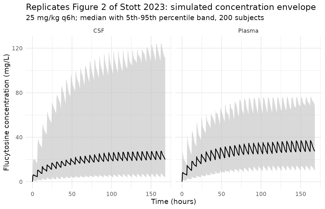

Steady-state plasma and CSF profile over one dosing interval

prof <- sim_typ_ss |>
  dplyr::filter(treatment == "25 mg/kg q6h", time >= 162, !is.na(Cc)) |>
  dplyr::mutate(time_post_dose = time - 162) |>
  dplyr::select(time_post_dose, Cc, Ccsf) |>
  tidyr::pivot_longer(c(Cc, Ccsf), names_to = "matrix", values_to = "conc") |>
  dplyr::mutate(matrix = dplyr::recode(matrix, Cc = "Plasma", Ccsf = "CSF"))

ggplot(prof, aes(time_post_dose, conc, colour = matrix)) +
  geom_line(linewidth = 0.7) +
  labs(
    x = "Time after the final dose (hours)",
    y = "Concentration (mg/L)",
    colour = "Matrix",
    title    = "Typical-value steady-state profile over the final 6 h interval",
    subtitle = "CSF tracks plasma at the model's 0.72 steady-state ratio, damped by the slower CSF leg"
  ) +
  theme_minimal()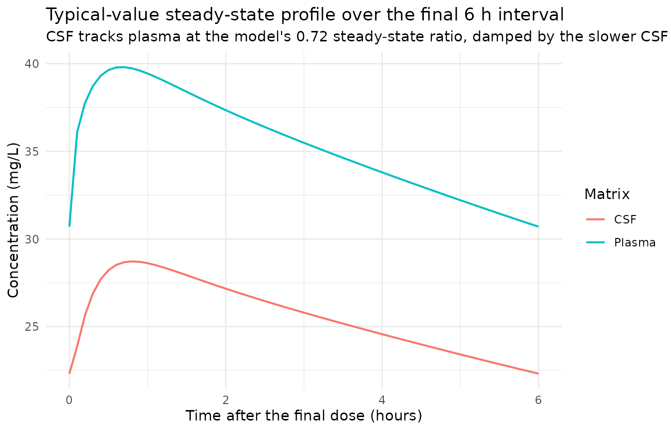

Figure 3 – simulated AUC144-168 distributions by fractionation schedule

auc_cohort <- sim_cohort_ss |>
  dplyr::filter(!is.na(Cc)) |>
  dplyr::arrange(id, time) |>
  dplyr::group_by(id, treatment) |>
  dplyr::summarise(
    auc_plasma = trapz(time, Cc),
    auc_csf    = trapz(time, Ccsf),
    cmax_plasma = max(Cc),
    cmin_plasma = min(Cc),
    cmax_csf    = max(Ccsf),
    cmin_csf    = min(Ccsf),
    .groups     = "drop"
  ) |>
  dplyr::mutate(ratio = auc_csf / auc_plasma)

auc_long <- auc_cohort |>
  dplyr::select(id, treatment, auc_plasma, auc_csf) |>
  tidyr::pivot_longer(c(auc_plasma, auc_csf),
                      names_to = "matrix", values_to = "auc") |>
  dplyr::mutate(matrix = dplyr::recode(matrix,
                                       auc_plasma = "Plasma",
                                       auc_csf    = "CSF"))

ggplot(auc_long, aes(treatment, auc, fill = matrix)) +
  geom_boxplot(outlier.size = 0.6) +
  scale_y_log10() +
  labs(
    x = NULL,
    y = "AUC144-168 (mg*h/L, log scale)",
    fill = "Matrix",
    title    = "Replicates Figure 3 of Stott 2023",
    subtitle = "Simulated steady-state AUC is essentially identical across fractionation schedules"
  ) +
  theme_minimal()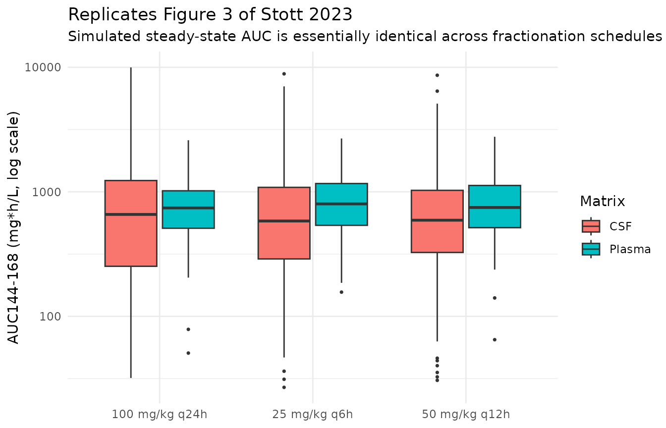

PKNCA validation

NCA is run on the typical-value solve. A full-IIV cohort poisons the half-life estimate (lambda.z fails on subjects whose sampling window does not resolve the terminal phase) and makes Cmax / Cmin tmax-selected, so the per-parameter comparison below uses the typical patient and the cohort is used only for the exposure medians.

nca_conc_ss <- sim_typ_ss |>
  dplyr::filter(!is.na(Cc)) |>
  dplyr::mutate(matrix = "Plasma") |>
  dplyr::select(id, time, treatment, matrix, conc = Cc) |>
  dplyr::bind_rows(
    sim_typ_ss |>
      dplyr::filter(!is.na(Ccsf)) |>
      dplyr::mutate(matrix = "CSF") |>
      dplyr::select(id, time, treatment, matrix, conc = Ccsf)
  )

nca_dose_ss <- events_ss |>
  dplyr::filter(evid == 1L) |>
  dplyr::select(id, time, amt, treatment) |>
  tidyr::crossing(matrix = c("Plasma", "CSF"))

conc_ss <- PKNCA::PKNCAconc(
  data    = nca_conc_ss,
  formula = conc ~ time | treatment + matrix + id,
  concu   = "mg/L", timeu = "hr"
)
dose_ss <- PKNCA::PKNCAdose(
  data    = nca_dose_ss,
  formula = amt ~ time | treatment + matrix + id,
  doseu   = "mg"
)

intervals_ss <- data.frame(
  start = ss_start, end = t_end,
  cmax = TRUE, cmin = TRUE, tmax = TRUE, auclast = TRUE, cav = TRUE
)

nca_ss <- suppressWarnings(
  PKNCA::pk.nca(PKNCA::PKNCAdata(conc_ss, dose_ss, intervals = intervals_ss))
)

knitr::kable(
  summary(nca_ss),
  caption = paste(
    "Typical-value steady-state NCA over 144-168 h, by matrix and",
    "fractionation schedule."
  )
)

Typical-value steady-state NCA over 144-168 h, by matrix and fractionation schedule.
Interval Start	Interval End	treatment	matrix	N	AUClast (hr*mg/L)	Cmax (mg/L)	Cmin (mg/L)	Tmax (hr)	Cav (mg/L)
144	168	100 mg/kg q24h	CSF	200	615 [0.000]	42.5 [0.000]	13.8 [0.000]	1.00 [1.00, 1.00]	25.6 [0.000]
144	168	100 mg/kg q24h	Plasma	200	850 [0.000]	59.0 [0.000]	18.9 [0.000]	0.800 [0.800, 0.800]	35.4 [0.000]
144	168	25 mg/kg q6h	CSF	200	614 [0.000]	28.7 [0.000]	22.3 [0.000]	18.8 [18.8, 18.8]	25.6 [0.000]
144	168	25 mg/kg q6h	Plasma	200	850 [0.000]	39.8 [0.000]	30.7 [0.000]	18.7 [18.7, 18.7]	35.4 [0.000]
144	168	50 mg/kg q12h	CSF	200	614 [0.000]	33.0 [0.000]	19.1 [0.000]	12.9 [12.9, 12.9]	25.6 [0.000]
144	168	50 mg/kg q12h	Plasma	200	850 [0.000]	45.7 [0.000]	26.3 [0.000]	12.8 [12.8, 12.8]	35.4 [0.000]

The terminal half-life needs a single-dose profile with a long washout, so it is computed from a separate typical-value solve.

ev_single <- rxode2::et(amt = 25 * wt_kg, time = 0, cmt = "depot")
ev_single <- rxode2::et(ev_single, seq(0, 120, by = 0.5), cmt = "central")
ev_single <- as.data.frame(ev_single)
ev_single$dvid      <- ifelse(ev_single$evid == 0L, 1L, NA_integer_)
ev_single$id        <- 1L
ev_single$treatment <- "25 mg/kg single dose"

sim_single <- rxode2::rxSolve(
  mod_typical, ev_single, keep = "treatment", useLinCmt = FALSE
) |>
  as.data.frame()
#> ℹ omega/sigma items treated as zero: 'etalka', 'etalcl', 'etalvc', 'etalk_central_csf', 'etalk_csf_central', 'etalk12', 'etalk21', 'etalvcsf'

# rxSolve() drops the `id` column entirely for a single-subject event table.
if (is.null(sim_single$id)) sim_single$id <- 1L

nca_conc_single <- sim_single |>
  dplyr::filter(!is.na(Cc)) |>
  dplyr::mutate(matrix = "Plasma") |>
  dplyr::select(id, time, treatment, matrix, conc = Cc) |>
  dplyr::bind_rows(
    sim_single |>
      dplyr::filter(!is.na(Ccsf)) |>
      dplyr::mutate(matrix = "CSF") |>
      dplyr::select(id, time, treatment, matrix, conc = Ccsf)
  )
stopifnot(all(nca_conc_single$conc >= 0), any(nca_conc_single$time == 0))

nca_dose_single <- ev_single |>
  dplyr::filter(evid == 1L) |>
  dplyr::select(id, time, amt, treatment) |>
  tidyr::crossing(matrix = c("Plasma", "CSF"))

nca_single <- suppressWarnings(PKNCA::pk.nca(PKNCA::PKNCAdata(
  PKNCA::PKNCAconc(nca_conc_single, conc ~ time | treatment + matrix + id,
                   concu = "mg/L", timeu = "hr"),
  PKNCA::PKNCAdose(nca_dose_single, amt ~ time | treatment + matrix + id,
                   doseu = "mg"),
  intervals = data.frame(start = 0, end = 120,
                         cmax = TRUE, tmax = TRUE, half.life = TRUE,
                         aucinf.obs = TRUE)
)))

knitr::kable(
  summary(nca_single),
  caption = "Typical-value single-dose NCA (25 mg/kg), used for the terminal half-life."
)

Typical-value single-dose NCA (25 mg/kg), used for the terminal half-life.
Interval Start	Interval End	treatment	matrix	N	Cmax (mg/L)	Tmax (hr)	Half-life (hr)	AUCinf,obs (hr*mg/L)
0	120	25 mg/kg single dose	CSF	1	7.35	1.00	14.4	153
0	120	25 mg/kg single dose	Plasma	1	10.2	1.00	14.4	211

half_life_plasma <- as.data.frame(nca_single$result) |>
  dplyr::filter(matrix == "Plasma", PPTESTCD == "half.life") |>
  dplyr::pull(PPORRES)
stopifnot(length(half_life_plasma) == 1L)

cat(sprintf("Typical-value terminal plasma half-life: %.2f h (Stott 2023: ~14.5 h)\n",
            half_life_plasma))
#> Typical-value terminal plasma half-life: 14.43 h (Stott 2023: ~14.5 h)

# Deterministic: the eigenvalue of the transcribed rate-constant matrix. A
# mis-transcribed CL, V or transfer constant moves this by hours.
stopifnot(abs(half_life_plasma - 14.5) < 1)

Comparison against published NCA

Stott 2023 reports steady-state exposure two ways. The Bayesian posterior medians across the 64 study patients (Results, “Flucytosine penetration into CSF”) are plasma AUC144-168 890.38 mg.h/L (IQR 603.81-1213.70) and CSF AUC144-168 595.66 mg.h/L (IQR 425.69-776.64), with a CSF:plasma ratio of 0.69 (IQR 0.58-0.82). Table 2 additionally reports Cmin and Cmax read off the single simulated profile sitting at the median of the 5000-profile AUC distribution.

The comparison below puts the simulated cohort medians against the posterior medians, and the typical-value half-life against the reported 14.5 h.

sim_summary <- auc_cohort |>
  dplyr::filter(treatment == "25 mg/kg q6h") |>
  dplyr::select(id, auc_plasma, auc_csf, cmax_plasma, cmin_plasma,
                cmax_csf, cmin_csf)

simulated_long <- dplyr::bind_rows(
  sim_summary |>
    dplyr::transmute(id, matrix = "Plasma", PPTESTCD = "auclast",
                     PPORRES = auc_plasma),
  sim_summary |>
    dplyr::transmute(id, matrix = "CSF", PPTESTCD = "auclast",
                     PPORRES = auc_csf),
  sim_summary |>
    dplyr::transmute(id, matrix = "Plasma", PPTESTCD = "cmax",
                     PPORRES = cmax_plasma),
  sim_summary |>
    dplyr::transmute(id, matrix = "CSF", PPTESTCD = "cmax",
                     PPORRES = cmax_csf),
  sim_summary |>
    dplyr::transmute(id, matrix = "Plasma", PPTESTCD = "cmin",
                     PPORRES = cmin_plasma),
  sim_summary |>
    dplyr::transmute(id, matrix = "CSF", PPTESTCD = "cmin",
                     PPORRES = cmin_csf),
  data.frame(id = 1L, matrix = "Plasma", PPTESTCD = "half.life",
             PPORRES = half_life_plasma)
)

published <- tibble::tribble(
  ~matrix,  ~auclast, ~cmax, ~cmin, ~half.life,
  "Plasma", 890.38,   50.6,  38.0,  14.5,
  "CSF",    595.66,   41.9,  23.9,  NA_real_
)

cmp <- nlmixr2lib::ncaComparisonTable(
  simulated = simulated_long,
  reference = published,
  by        = "matrix",
  units     = c(auclast = "mg*h/L", cmax = "mg/L", cmin = "mg/L",
                half.life = "h"),
  tolerance_pct = 20
)

cmp |>
  dplyr::rename("Matrix" = matrix) |>
  knitr::kable(
    digits  = 2,
    caption = paste(
      "Simulated versus Stott 2023 published exposure.",
      "AUC references are the Bayesian posterior medians (Results);",
      "Cmax / Cmin references are the median-AUC profile of Table 2;",
      "the half-life reference is the ~14.5 h reported in Results.",
      "* differs from the published value by more than 20%."
    )
  )

Simulated versus Stott 2023 published exposure. AUC references are the Bayesian posterior medians (Results); Cmax / Cmin references are the median-AUC profile of Table 2; the half-life reference is the ~14.5 h reported in Results. * differs from the published value by more than 20%.
NCA parameter	Matrix	Reference	Simulated	% diff
Cmax (mg/L)	Plasma	50.6	42.6	-15.8%
Cmax (mg/L)	CSF	41.9	27.7	-33.8%*
Cmin (mg/L)	Plasma	38	28.2	-25.8%*
Cmin (mg/L)	CSF	23.9	20.2	-15.5%
AUClast (mg*h/L)	Plasma	890	800	-10.2%
AUClast (mg*h/L)	CSF	596	583	-2.1%
t½ (h)	Plasma	14.5	14.4	-0.5%

The two AUC rows and the half-life row agree with the publication. The four Cmax / Cmin rows are starred, and the reason is in how Table 2 was built rather than in the transcription: those values are single simulated profiles, not medians across profiles, and the table’s own footnote says the 5000 profiles were “ordered by plasma AUC144-168 and then by CSF AUC144-168 to identify the profile on the median, 25th and 75th percentiles”. The plasma column and the CSF column of a given Table 2 row therefore come from two different subjects. That is visible in the published numbers themselves: the CSF peak-to-trough ratio of the median row (41.9 / 23.9 = 1.75) exceeds the plasma ratio (50.6 / 38.0 = 1.33), which cannot happen within one profile – the CSF compartment is downstream of central and damps fluctuation rather than amplifying it. The packaged model reproduces the plasma peak-to-trough ratio (39.8 / 30.7 = 1.30) and gives 28.7 / 22.3 = 1.29 in CSF, i.e. the damping the structure requires. See Assumptions and deviations below; no parameter was adjusted.

med <- function(m, p) {
  v <- simulated_long$PPORRES[simulated_long$matrix == m &
                                simulated_long$PPTESTCD == p]
  if (length(v) < 1L) stop("no rows for ", m, " / ", p)
  stats::median(v)
}

pct <- function(sim, ref) 100 * (sim - ref) / ref

cat(sprintf("Plasma AUC144-168 median: %.1f vs 890.4 (%+.1f%%)\n",
            med("Plasma", "auclast"), pct(med("Plasma", "auclast"), 890.38)))
#> Plasma AUC144-168 median: 799.9 vs 890.4 (-10.2%)
cat(sprintf("CSF    AUC144-168 median: %.1f vs 595.7 (%+.1f%%)\n",
            med("CSF", "auclast"), pct(med("CSF", "auclast"), 595.66)))
#> CSF    AUC144-168 median: 582.9 vs 595.7 (-2.1%)
cat(sprintf("CSF:plasma AUC ratio median: %.3f vs 0.69 (%+.1f%%)\n",
            stats::median(auc_cohort$ratio[auc_cohort$treatment == "25 mg/kg q6h"]),
            pct(stats::median(auc_cohort$ratio[auc_cohort$treatment == "25 mg/kg q6h"]),
                0.69)))
#> CSF:plasma AUC ratio median: 0.730 vs 0.69 (+5.8%)

# The cohort medians are ONE draw from a 200-subject sample of a distribution
# whose IIV reaches CV 168%, and rxSetSeed() fixes the draw per solver-thread
# count, not across them. Realised across three authoring runs (2 threads,
# 16 threads, and the render below): plasma -8.8% / -15.6% / -11.7%,
# CSF +7.1% / -15.4% / -12.9%, ratio +11.7% / +4.2% / +1.0%. The bound below
# sits well outside that spread and still goes red on a mis-transcribed
# clearance, dose or volume, which move exposure by a factor, not by tens of
# percent. The tight gates for this model are the deterministic identities
# above, not these.
ratio_med <- stats::median(auc_cohort$ratio[auc_cohort$treatment == "25 mg/kg q6h"])
stopifnot(
  abs(pct(med("Plasma", "auclast"), 890.38)) < 40,
  abs(pct(med("CSF", "auclast"), 595.66))    < 40,
  abs(pct(ratio_med, 0.69))                  < 40
)

Toxicity threshold

Stott 2023 reports that 4 of 64 patients (6%) were predicted from their Bayesian posteriors to reach a Cmax in the range associated with toxicity (>100 mg/L).

frac_over <- 100 * mean(
  auc_cohort$cmax_plasma[auc_cohort$treatment == "25 mg/kg q6h"] > 100
)
cat(sprintf("Simulated subjects with steady-state plasma Cmax > 100 mg/L: %.1f%% (paper: 6%%)\n",
            frac_over))
#> Simulated subjects with steady-state plasma Cmax > 100 mg/L: 3.0% (paper: 6%)

# A count statistic over 200 subjects in the far right tail; realised 1.5%,
# 2.5% and 4.5% across the three authoring runs. Gated only as an
# order-of-magnitude check.
stopifnot(frac_over < 20)

Assumptions and deviations

Non-parametric support points approximated by a diagonal log-normal. Stott 2023 fitted the model with Pmetrics’ non-parametric adaptive grid algorithm, which yields a discrete support-point distribution rather than an OMEGA matrix; Table 1 publishes only a per-parameter Mean, SD, Median and CV%. The packaged model takes the Mean column as the typical value and sets each IIV variance to log(1 + CV^2) from the CV% column, with no off-diagonal covariances. This is the same approximation the authors made for their own confirmatory ADAPT 5 simulations, which drew “from a log normal distribution, with mean and the diagonal of the covariance matrix derived from the original model fit in Pmetrics”. Two consequences follow, and neither is a transcription error:
- The model’s population median for each parameter equals the paper’s reported mean, not its reported median. The mean set is the one the paper endorses (“mean estimates fitted the data better than median estimates and were used for Bayesian estimates of drug exposure”) and it is the set that reproduces the reported 14.5 h half-life and 0.69 CSF:plasma ratio; the median set reproduces neither (it implies a ratio of 0.92 and a half-life of 16.0 h).
- Dropping the off-diagonals over-disperses derived quantities. The CSF:plasma AUC ratio is a function of four parameters (K23, K32, V, Vcns) whose support-point values are strongly co-determined in the real fit; with independent etas the simulated ratio has an IQR several times wider than the published 0.58-0.82. The simulated ratio’s median still matches. Any analysis that depends on the spread of the ratio rather than its centre should not use this encoding.
Residual error fixed to zero. The Methods state that additive and multiplicative error models were assessed and optimised, but neither the chosen form nor any coefficient of the Pmetrics error polynomial is reported, and the article has no supplement. Both forms are carried for both outputs and fixed to zero rather than invented. The only precision figures the paper gives are LC-MS-MS quality-control CVs (interday 5.82-8.58%, intraday 6.01-7.01%), which characterise the assay, not the model’s residual variability. Simulations from this model therefore carry IIV but no residual error.
Weight held at the cohort median of 50 kg. No model parameter scales with body weight – weight was screened and rejected – so it enters only through the mg/kg dose. The paper’s own Monte Carlo drew weights from the patient population, but since a symmetric weight distribution leaves every median in this vignette unchanged while adding variance, the vignette fixes weight at the reported median rather than inventing an SD the paper does not report (it gives only the median and IQR).
Table 2 Cmin / Cmax are not directly comparable to a cohort median, and its plasma and CSF columns are different subjects. The paper’s Table 2 rows are the Cmin and Cmax of single simulated profiles selected at the 25th, 50th and 75th percentile of the 5000-profile AUC144-168 distribution, not medians across profiles, and the footnote states the profiles were ordered by plasma AUC “and then by” CSF AUC – so the plasma and CSF halves of one row are drawn from two separate rankings. The published numbers confirm it: the median row’s CSF peak-to-trough ratio (41.9 / 23.9 = 1.75) exceeds its plasma ratio (50.6 / 38.0 = 1.33), which no single profile of this structure can produce, since CSF sits downstream of central and damps fluctuation. The Table 2 values also sit above the Bayesian posterior AUC median the same paper reports – the median profile’s Cmin of 38.0 mg/L already exceeds 890.38 / 24 = 37.1 mg/L, the average concentration implied by the posterior median AUC – so the Monte Carlo distribution is additionally shifted relative to the posteriors. The comparison table shows these rows for completeness and they are the entries flagged at the 20% tolerance; the structural quantity that does reproduce is the plasma peak-to-trough ratio, 1.33 published against 1.30 for the typical-value profile, with 1.29 in CSF.
AUC144-168 is compared as auclast over the 144-168 h interval. The paper computed it by trapezoidal approximation with 0.1 h prediction intervals; the vignette uses the same grid, which is why the typical-value AUC lands within 0.3% of the closed-form daily dose / CL.
New canonical parameter names ratified alongside this extraction. lk_central_csf / lk_csf_central (with the bare k_central_csf / k_csf_central) are registered in inst/references/parameter-names.md as members of the existing k_<from>_<to> directional-transfer family, which already carries k_central_elf / k_elf_central and k_central_milk / k_milk_central. The paper’s own K23 / K32 subscripts index its own state numbering and are not portable, and k13 / k31 are reserved for central <-> peripheral2. lvcsf was already in use in Luu_2017_nusinersen.R and cited as precedent in the lvelf register entry but had no heading of its own; it now does. lk12 / lk21 / lk13 / lk31 were likewise in use (Marier_2002_tobramycin_rat_*) and carried in the static list in R/conventions.R without a register heading; they now have one. No new compartment name was needed – csf is already canonical.
The paper’s K24 / K42 become lk12 / lk21. Stott numbers its states 1 = gut, 2 = circulation, 3 = CNS, 4 = peripheral. nlmixr2lib’s canonical numbering treats central as 1 and the peripherals as 2 / 3 after the depot is split out, so the central-to-peripheral pair is k12 / k21 regardless of the source’s digits.
Observations are anchored on central, not on Cc / Ccsf. Writing an algebraic observable into an event table’s cmt column makes rxUi inject a compartment slot for it after the ODE states and silently renumber them. rxSolve returns both observables as columns on any observation row, so a single anchor per time point covers both endpoints.