R- and S-citalopram + desmethylcitalopram (Akil 2016)
Source:vignettes/articles/Akil_2016_citalopram.Rmd
Akil_2016_citalopram.RmdModel and source
- Citation: Akil A, Bies RR, Pollock BG, Avramopoulos D, Devanand DP, Mintzer JE, Porsteinsson AP, Schneider LS, Weintraub D, Yesavage J, Shade DM, Lyketsos CG. A population pharmacokinetic model for R- and S-citalopram and desmethylcitalopram in Alzheimer’s disease patients with agitation. J Pharmacokinet Pharmacodyn. 2016 Feb;43(1):99-109. doi:10.1007/s10928-015-9457-6
- Description: Joint enantiomer-resolved parent-plus-metabolite population PK model for racemic citalopram in elderly Alzheimer’s disease patients treated for agitation in the CitAD trial (Akil 2016). Four disposition compartments, one per measured analyte – R-citalopram, S-citalopram, R-desmethylcitalopram and S-desmethylcitalopram – fed by a single oral depot whose first-order absorption rate constant Ka is shared by the two enantiomers and fixed at 1 /h. The racemic capsule splits 50/50 into the two parent compartments. Parent-to-metabolite conversion is complete, so the apparent metabolic clearance of each parent is also its formation clearance into the corresponding desmethyl metabolite, and each metabolite is assumed to share the apparent volume of distribution of its parent enantiomer. Clearance of the R-enantiomer is slower than that of the S-enantiomer. Covariate effects differ by enantiomer: R-citalopram apparent metabolic clearance falls with age and is about 30 percent lower in women; S-citalopram apparent metabolic clearance falls with age, rises with body weight and is about 36 percent higher in CYP2C19 extensive/rapid metabolizers than in intermediate/poor metabolizers; both desmethylcitalopram clearances rise with body weight. All clearances and volumes are apparent (divided by the unknown oral bioavailability F).
- Article: https://doi.org/10.1007/s10928-015-9457-6
Akil 2016 is a joint, enantiomer-resolved, parent-plus-metabolite population PK analysis of racemic citalopram in the Citalopram for Agitation in Alzheimer’s Disease (CitAD) trial. Four analytes were measured by chiral HPLC and fitted simultaneously: R-citalopram, S-citalopram (escitalopram), and their N-desmethyl metabolites R- and S-desmethylcitalopram. The clinical interest is that the two enantiomers are not pharmacologically equivalent – the paper cites evidence that R-citalopram counteracts S-citalopram activity, and that R-citalopram exposure drives QTc prolongation and cognitive decline in this population – so a model that resolves them separately is a prerequisite for any exposure-response analysis in agitated Alzheimer’s disease patients.
Population
Ninety-four CitAD participants received citalopram and provided plasma samples; 81 contributed to the population analysis (Akil 2016 Results, “Patient characteristics”). The cohort was 41 male / 40 female (50.6 / 49.4 percent), mean age 77.8 years (SD 8.2, range 47-90), mean weight 71.5 kg (SD 17.2, range 40-122.3) and mean body mass index 26.3 (SD 5.2, range 15.4-41.6). CYP2C19 genotype was extensive in 43 (53.1 percent), rapid in 3 (3.7 percent), intermediate in 17 (21 percent) and poor in 3 (3.7 percent); it was missing in 15 (18.5 percent), and the paper carried those subjects as their own covariate level rather than imputing them.
Dosing was oral racemic citalopram, started at 10 mg once daily and titrated over two weeks to a 30 mg once-daily target given as three 10 mg capsules in the morning. Sampling was sparse and at steady state – weeks 3, 6 and 9 – giving 2.5, 2.5, 2.2 and 1.3 observations per subject for R-citalopram, S-citalopram, R-desmethylcitalopram and S-desmethylcitalopram respectively (Akil 2016 Table 1). The limit of quantitation was 5 ng/mL for every analyte except S-desmethylcitalopram, where it was 10 ng/mL.
The same information is available programmatically via the model’s
population metadata
(readModelDb("Akil_2016_citalopram")()$population).
Source trace
The per-parameter origin is recorded as an in-file comment next to
each ini() entry in
inst/modeldb/specificDrugs/Akil_2016_citalopram.R. The
table below collects them in one place for review.
| Equation / parameter | Value | Source location |
|---|---|---|
d/dt(central_r_enant),
d/dt(central_s_enant)
|
n/a | Akil 2016 equations (1) and (2) |
d/dt(central_dcit_r_enant),
d/dt(central_dcit_s_enant)
|
n/a | Akil 2016 equations (3) and (4) |
| Four compartments, one per compound; complete parent-to-metabolite conversion | n/a | Akil 2016 Results, “Population pharmacokinetic modeling” and Fig. 3 |
Shared ka; shared volume for parent and metabolite of
each enantiomer |
n/a | Akil 2016 Results, “Population pharmacokinetic modeling” |
| 50/50 racemic split of the capsule dose | 0.5 | Akil 2016 Discussion (“citalopram is administered as 50/50 racemic mixture”) |
lka |
1 /h (fixed) | Table 3, Ka, h-1 = 1 (Fixed), both blocks |
lcl_r_enant |
13 L/h | Table 3, CL Rp /F for male, L/h
|
e_sexf_cl_r_enant |
9.05 / 13 | Table 3, CL Rp /F for female, L/h = 9.05 |
lvc_r_enant |
1830 L | Table 3, R block V/F, L
|
lcl_dcit_r_enant |
24.4 L/h | Table 3, CL Rm /F, L/h
|
lcl_s_enant |
22.1 L/h | Table 3, CL Sp /F for EM/RM, L/h
|
e_cyp2c19_im_cl_s_enant,
e_cyp2c19_pm_cl_s_enant
|
16.3 / 22.1 | Table 3, CL Sp /F for IM/PM, L/h = 16.3 |
e_cyp2c19_missing_cl_s_enant |
16.8 / 22.1 | Table 3, CL Sp /F for Missing, L/h = 16.8 |
lvc_s_enant |
1390 L | Table 3, S block V/F, L
|
lcl_dcit_s_enant |
38.8 L/h | Table 3, CL Sm /F, L/h
|
e_age_cl_r_enant |
-0.822 | Results, CLRp/F = CL0/F x (Age/60)^-0.822
|
e_age_cl_s_enant |
-1.33 | Results, CLSp/F = CL0/F x (Age/60)^-1.33
|
e_wt_cl_s_enant |
0.75 | Results, CLSp/F = CL0/F x (WT/70)^0.75
|
e_wt_cl_dcit_r_enant,
e_wt_cl_dcit_s_enant
|
0.75 | Results, CLm/F = CL0/F x (WT/70)^0.75
|
| Age centring 60 y; weight centring 70 kg | n/a | Methods, “Final model” |
etalcl_r_enant, etalvc_r_enant,
etalcl_dcit_r_enant
|
26.38, 166.73, 30.61 % CV | Table 3, R block omega rows |
etalcl_s_enant + etalvc_s_enant block |
38.34, 47.1, 75.37 % | Table 3, S block omega rows |
etalcl_dcit_s_enant |
20.49 % CV | Table 3, S block x CLm , %
|
addSd_r_enant |
13.42 ng/mL | Table 3, R block sigma row, “ng/ml (additive)” |
propSd_dcit_r_enant |
21.54 % | Table 3, R block sigma row, “% (proportional)” |
propSd_s_enant, propSd_dcit_s_enant
|
21.61 % | Table 3, S block sigma row, “% (proportional)” |
Akil 2016’s Table 3 renders the Greek omega and sigma symbols as the
Latin letters “x” and “r” in the published PDF’s text layer; the row
labels quoted in the model file’s ini() comments preserve
that mangling verbatim, while this table spells the intended symbols
out.
mod <- readModelDb("Akil_2016_citalopram")
ui <- rxode2::rxode(mod)
#> ℹ parameter labels from comments will be replaced by 'label()'

analytes <- tibble::tribble(
  ~column,            ~analyte,
  "Cc_r_enant",       "R-citalopram",
  "Cc_s_enant",       "S-citalopram",
  "Cc_dcit_r_enant",  "R-desmethylcitalopram",
  "Cc_dcit_s_enant",  "S-desmethylcitalopram"
)

# The ODE states, in declaration order. Observation rows in every event table
# below point at an ODE STATE (never at an algebraic observable such as
# `Cc_r_enant`), and carry an explicit `dvid` because the model declares four
# residual-error endpoints.
ui$state
#> [1] "depot"                "central_r_enant"      "central_s_enant"
#> [4] "central_dcit_r_enant" "central_dcit_s_enant"
Virtual cohort
Original CitAD concentration data are not public. The cohort below reproduces the Akil 2016 Table 1 marginal distributions: 81 subjects, age and weight drawn from truncated normals matching the reported mean, SD and range, sex split 41 male / 40 female, and CYP2C19 phenotype counts 43 / 3 / 17 / 3 / 15 for EM / RM / IM / PM / missing. Covariates are drawn independently because Akil 2016 reports only marginal distributions.
# `set.seed()` seeds R's RNG (the covariate draws below). It does NOT seed
# rxode2's simulation RNG, whose streams are partitioned per solver thread --
# so the eta draws differ between this machine and a CI runner with a different
# thread count. Every assertion below is therefore written on medians and
# robust quantiles, never on an extreme or an exact value.
set.seed(20160126)

n_subj <- 81L

rtruncnorm1 <- function(n, mean, sd, lo, hi) {
  x <- rnorm(n, mean, sd)
  while (any(bad <- x < lo | x > hi)) x[bad] <- rnorm(sum(bad), mean, sd)
  x
}

# Akil 2016 Table 1 CYP2C19 counts; EM and RM are the model's reference level.
pheno <- rep(c("EM", "RM", "IM", "PM", "Missing"), times = c(43L, 3L, 17L, 3L, 15L))
stopifnot(length(pheno) == n_subj)

subjects <- tibble(
  id   = seq_len(n_subj),
  AGE  = rtruncnorm1(n_subj, 77.8, 8.2, 47, 90),
  WT   = rtruncnorm1(n_subj, 71.5, 17.2, 40, 122.3),
  SEXF = sample(rep(c(0, 1), times = c(41L, 40L))),
  phenotype = sample(pheno)
) |>
  mutate(
    CYP2C19_IM      = as.numeric(phenotype == "IM"),
    CYP2C19_PM      = as.numeric(phenotype == "PM"),
    CYP2C19_MISSING = as.numeric(phenotype == "Missing"),
    # The model pools IM and PM into a single stratum, matching Akil 2016
    # Methods "Final model" (EM/RM = 1, IM/PM = 2, missing = 3).
    cyp_group = case_when(
      phenotype == "Missing"         ~ "Missing",
      phenotype %in% c("IM", "PM")   ~ "IM/PM",
      TRUE                           ~ "EM/RM"
    )
  )

stopifnot(
  nrow(subjects) == 81L,
  sum(subjects$SEXF) == 40L,
  sum(subjects$cyp_group == "EM/RM") == 46L,
  sum(subjects$cyp_group == "IM/PM") == 20L,
  sum(subjects$cyp_group == "Missing") == 15L
)

knitr::kable(
  subjects |>
    summarise(
      `N`                = n(),
      `Age, mean (SD)`   = sprintf("%.1f (%.1f)", mean(AGE), sd(AGE)),
      `Weight, mean (SD)` = sprintf("%.1f (%.1f)", mean(WT), sd(WT)),
      `Female, n (%)`    = sprintf("%d (%.1f%%)", sum(SEXF), 100 * mean(SEXF))
    ),
  caption = paste(
    "Simulated cohort against Akil 2016 Table 1 (N = 81; age 77.8 (8.2) y;",
    "weight 71.5 (17.2) kg; female 40 (49.4%))."
  )
)| N | Age, mean (SD) | Weight, mean (SD) | Female, n (%) |
|---|---|---|---|
| 81 | 76.7 (7.7) | 71.2 (14.8) | 40 (49.4%) |
Dosing and observation schedule
CitAD titrated to 30 mg once daily and sampled at weeks 3, 6 and 9.
The simulation gives 30 mg of the racemate once daily
for 63 days (through week 9) and observes the final dosing interval
densely. Because the dose record carries the racemic amount, each parent
compartment receives 15 mg – the 0.5 * split in the model
body.
tau       <- 24              # dosing interval, h
n_doses   <- 63L             # daily dosing through week 9 of CitAD
t_last    <- (n_doses - 1L) * tau
obs_grid  <- seq(t_last, t_last + tau, by = 0.25)

# Route A event table: `cmt` names an ODE STATE and observation rows carry an
# explicit `dvid`. rxSolve returns every algebraic observable as a column
# regardless of which endpoint the row is tagged with, so one dvid suffices to
# read all four analytes. Built as a plain data.frame -- rxode2::et() does not
# carry `dvid` through in the way this route needs.
events <- bind_rows(
  tidyr::crossing(subjects, time = seq(0, t_last, by = tau)) |>
    mutate(amt = 30, cmt = "depot", evid = 1L, dvid = NA_integer_),
  tidyr::crossing(subjects, time = obs_grid) |>
    mutate(amt = NA_real_, cmt = "central_r_enant", evid = 0L, dvid = 1L)
) |>
  arrange(id, time, desc(evid))

stopifnot(!anyDuplicated(unique(events[, c("id", "time", "evid")])))
Simulation
sim <- rxode2::rxSolve(
  mod,
  events = events,
  keep   = c("AGE", "WT", "SEXF", "cyp_group"),
  # rxode2's automatic ODE -> linCmt conversion corrupts the dvid -> cmt
  # mapping for multi-state, multi-endpoint models; disable it.
  useLinCmt = FALSE
) |>
  as.data.frame()
#> ℹ parameter labels from comments will be replaced by 'label()'

# `Cc_*` are the individual predictions (IPRED); residual error lives in `sim`
# / `ipredSim`. NCA below uses the IPRED columns, so no concentration can be
# driven negative by the residual and `auclast` is never NaN.
stopifnot(
  all(analytes$column %in% names(sim)),
  !anyNA(sim[, analytes$column]),
  all(sim[, analytes$column] >= 0)
)
A deterministic typical-value solve is used for the structural checks, because those are statements about the model’s equations rather than about a cohort.
mod_tv <- rxode2::zeroRe(mod)
#> ℹ parameter labels from comments will be replaced by 'label()'

# One typical subject per CYP2C19 stratum, at the model's own centring
# covariates (age 60 y, 70 kg, male) so the parameters are exactly the Table 3
# thetas, plus a long washout after the last dose for terminal-slope recovery.
tv_subjects <- tibble(
  id        = 1:3,
  cyp_group = c("EM/RM", "IM/PM", "Missing"),
  AGE = 60, WT = 70, SEXF = 0,
  CYP2C19_IM      = c(0, 1, 0),
  CYP2C19_PM      = 0,
  CYP2C19_MISSING = c(0, 0, 1)
)

tv_obs <- c(obs_grid, seq(t_last + tau, t_last + tau + 900, by = 2))

events_tv <- bind_rows(
  tidyr::crossing(tv_subjects, time = seq(0, t_last, by = tau)) |>
    mutate(amt = 30, cmt = "depot", evid = 1L, dvid = NA_integer_),
  tidyr::crossing(tv_subjects, time = unique(tv_obs)) |>
    mutate(amt = NA_real_, cmt = "central_r_enant", evid = 0L, dvid = 1L)
) |>
  arrange(id, time, desc(evid))

sim_tv <- rxode2::rxSolve(
  mod_tv, events = events_tv, keep = c("cyp_group"), useLinCmt = FALSE
) |>
  as.data.frame()
#> ℹ omega/sigma items treated as zero: 'etalcl_r_enant', 'etalvc_r_enant', 'etalcl_dcit_r_enant', 'etalcl_s_enant', 'etalvc_s_enant', 'etalcl_dcit_s_enant'
#> Warning: multi-subject simulation without without 'omega'
Structural check: complete parent-to-metabolite conversion
Akil 2016’s final model converts parent to metabolite
completely (Results, “Population pharmacokinetic modeling”).
That makes each analyte’s steady-state exposure over a dosing interval
exactly dose / CL, where dose is the
per-enantiomer 15 mg rather than the 30 mg racemic
capsule. This is the sharpest available gate on the ODE system: it fails
if the racemic split is wrong, if any mass leaks, or if a metabolite
clearance is divided by the wrong volume. Both sides use the same drawn
parameters, so the residual is pure numerical error and the tolerance is
tight.
trapz <- function(t, y) sum(diff(t) * (head(y, -1) + tail(y, -1)) / 2)

ss_tv <- sim_tv |> filter(cyp_group == "EM/RM", time >= t_last, time <= t_last + tau)
p_tv  <- sim_tv |> filter(cyp_group == "EM/RM") |> slice(1)

dose_enant <- 15  # mg of each enantiomer in a 30 mg racemic capsule

massbal <- tibble(
  analyte  = analytes$analyte,
  cl       = c(p_tv$cl_r_enant, p_tv$cl_s_enant,
               p_tv$cl_dcit_r_enant, p_tv$cl_dcit_s_enant),
  auc_sim  = vapply(analytes$column,
                    function(k) trapz(ss_tv$time, ss_tv[[k]]) / 1000,
                    numeric(1))
) |>
  mutate(
    auc_closed_form = dose_enant / cl,
    pct_diff        = 100 * (auc_sim - auc_closed_form) / auc_closed_form
  )

# Deterministic identity -- the only error is trapezoidal on a 0.25 h grid.
stopifnot(max(abs(massbal$pct_diff)) < 0.5)

massbal |>
  mutate(across(c(cl, auc_sim, auc_closed_form), ~round(., 4)),
         pct_diff = round(pct_diff, 4)) |>
  rename(
    "Analyte"                       = analyte,
    "CL/F (L/h)"                    = cl,
    "Simulated AUC0-tau (mg*h/L)"   = auc_sim,
    "15 mg / CL (mg*h/L)"           = auc_closed_form,
    "Difference (%)"                = pct_diff
  ) |>
  knitr::kable(
    caption = paste(
      "Steady-state exposure against the closed form implied by complete",
      "parent-to-metabolite conversion, typical CYP2C19 EM/RM subject at the",
      "model's centring covariates (60 y, 70 kg, male)."
    )
)| Analyte | CL/F (L/h) | Simulated AUC0-tau (mg*h/L) | 15 mg / CL (mg*h/L) | Difference (%) |
|---|---|---|---|---|
| R-citalopram | 13.0 | 1.1538 | 1.1538 | -0.0059 |
| S-citalopram | 22.1 | 0.6787 | 0.6787 | -0.0083 |
| R-desmethylcitalopram | 24.4 | 0.6147 | 0.6148 | -0.0047 |
| S-desmethylcitalopram | 38.8 | 0.3866 | 0.3866 | 0.0000 |
The per-enantiomer dose is not an assumption imposed here – it is recoverable from the paper. Akil 2016’s Discussion reports empirical-Bayes exposures of 1.46 +/- 0.58 mg*h/L for R-citalopram and 0.97 +/- 0.45 for S-citalopram against empirical-Bayes mean clearances of 8.73 and 13.76 L/h. Dividing a 15 mg per-enantiomer dose by those clearances gives 1.72 and 1.09 mg*h/L, within about 15 percent of the reported exposures; the 30 mg racemic dose would give 3.44 and 2.18, roughly twice the reported values. (The residual 15 percent is itself informative – see the Errata section on achieved dose.)
Replicate published covariate relationships
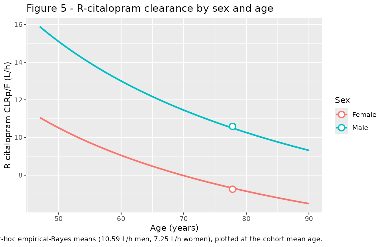
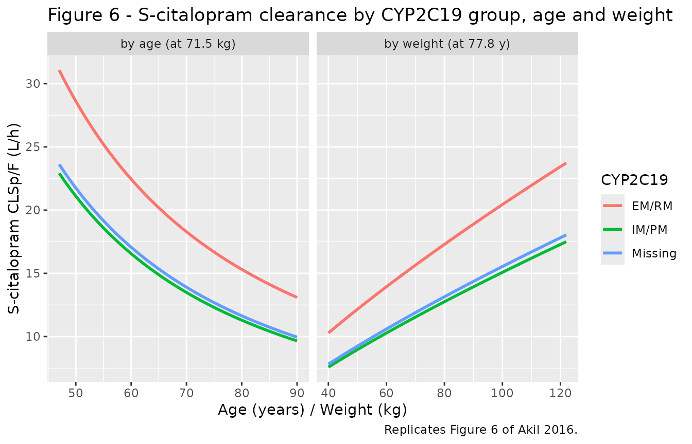
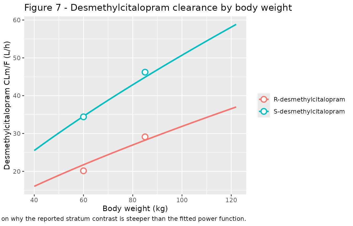
Akil 2016 Figs. 5-7 plot empirical-Bayes clearances against the retained covariates with the fitted covariate function overlaid. The panels below reproduce those fitted functions from the packaged model.
# Replicates Figure 5 of Akil 2016: R-citalopram apparent metabolic clearance
# by patient sex and age.
age_grid <- tibble(AGE = seq(47, 90, by = 0.5))

fig5 <- tidyr::crossing(age_grid, SEXF = c(0, 1)) |>
  mutate(
    Sex   = ifelse(SEXF == 1, "Female", "Male"),
    CL_Rp = 13 * (9.05 / 13)^SEXF * (AGE / 60)^-0.822
  )

ggplot(fig5, aes(AGE, CL_Rp, colour = Sex)) +
  geom_line(linewidth = 1) +
  geom_point(
    data = tibble(
      AGE = 77.8, CL_Rp = c(10.59, 7.25), Sex = c("Male", "Female")
    ),
    size = 3, shape = 21, fill = "white", stroke = 1.2
  ) +
  labs(
    x = "Age (years)", y = "R-citalopram CLRp/F (L/h)",
    title = "Figure 5 - R-citalopram clearance by sex and age",
    caption = paste(
      "Replicates Figure 5 of Akil 2016. Open points are the paper's reported",
      "post-hoc empirical-Bayes means (10.59 L/h men, 7.25 L/h women),",
      "plotted at the cohort mean age."
    )
  )
# Replicates Figure 6 of Akil 2016: S-citalopram apparent metabolic clearance
# by CYP2C19 genotype group, age and body weight.
cyp_ratio <- c("EM/RM" = 1, "IM/PM" = 16.3 / 22.1, "Missing" = 16.8 / 22.1)

fig6_age <- tidyr::crossing(age_grid, cyp_group = names(cyp_ratio)) |>
  mutate(CL_Sp = 22.1 * cyp_ratio[cyp_group] * (AGE / 60)^-1.33 * (71.5 / 70)^0.75,
         panel = "by age (at 71.5 kg)", x = AGE)

fig6_wt <- tidyr::crossing(tibble(WT = seq(40, 122.3, by = 0.5)),
                           cyp_group = names(cyp_ratio)) |>
  mutate(CL_Sp = 22.1 * cyp_ratio[cyp_group] * (77.8 / 60)^-1.33 * (WT / 70)^0.75,
         panel = "by weight (at 77.8 y)", x = WT)

bind_rows(fig6_age, fig6_wt) |>
  ggplot(aes(x, CL_Sp, colour = cyp_group)) +
  geom_line(linewidth = 1) +
  facet_wrap(~panel, scales = "free_x") +
  labs(
    x = "Age (years) / Weight (kg)", y = "S-citalopram CLSp/F (L/h)",
    colour = "CYP2C19",
    title = "Figure 6 - S-citalopram clearance by CYP2C19 group, age and weight",
    caption = "Replicates Figure 6 of Akil 2016."
  )
# Replicates Figure 7 of Akil 2016: R- and S-desmethylcitalopram apparent
# clearance by body weight.
fig7 <- tidyr::crossing(
  tibble(WT = seq(40, 122.3, by = 0.5)),
  tibble(analyte = c("R-desmethylcitalopram", "S-desmethylcitalopram"),
         cl0     = c(24.4, 38.8))
) |>
  mutate(CLm = cl0 * (WT / 70)^0.75)

ggplot(fig7, aes(WT, CLm, colour = analyte)) +
  geom_line(linewidth = 1) +
  geom_point(
    data = tibble(
      WT      = rep(c(60, 85), 2),
      CLm     = c(20.14, 29.12, 34.41, 46.22),
      analyte = rep(c("R-desmethylcitalopram", "S-desmethylcitalopram"), each = 2)
    ),
    size = 3, shape = 21, fill = "white", stroke = 1.2
  ) +
  labs(
    x = "Body weight (kg)", y = "Desmethylcitalopram CLm/F (L/h)", colour = NULL,
    title = "Figure 7 - Desmethylcitalopram clearance by body weight",
    caption = paste(
      "Replicates Figure 7 of Akil 2016. Open points are the paper's reported",
      "empirical-Bayes means for the < 70 kg and >= 70 kg strata, plotted at",
      "nominal 60 and 85 kg; see the Errata note on why the reported stratum",
      "contrast is steeper than the fitted power function."
    )
  )
Typical values against the paper’s empirical-Bayes means
Evaluating the model at the cohort’s mean covariates should land near the paper’s reported post-hoc empirical-Bayes means. This is a non-circular check: those means are computed from the individual fits and reported in the Discussion, not in the parameter table the model was transcribed from.
tv_at <- function(SEXF, IM, MISS, AGE = 77.8, WT = 71.5) {
  ev <- data.frame(
    time = c(0, 1), amt = c(30, NA_real_), cmt = c("depot", "central_r_enant"),
    evid = c(1L, 0L), dvid = c(NA_integer_, 1L),
    AGE = AGE, WT = WT, SEXF = SEXF,
    CYP2C19_IM = IM, CYP2C19_PM = 0, CYP2C19_MISSING = MISS
  )
  rxode2::rxSolve(mod_tv, ev, returnType = "data.frame", useLinCmt = FALSE)[1, ]
}

# S-citalopram: weight the three CYP2C19 strata by their cohort frequencies
# (46 / 20 / 15 of 81), because the paper's empirical-Bayes mean pools them.
s_strata <- rbind(tv_at(0, 0, 0), tv_at(0, 1, 0), tv_at(0, 0, 1))
#> ℹ omega/sigma items treated as zero: 'etalcl_r_enant', 'etalvc_r_enant', 'etalcl_dcit_r_enant', 'etalcl_s_enant', 'etalvc_s_enant', 'etalcl_dcit_s_enant'
#> ℹ omega/sigma items treated as zero: 'etalcl_r_enant', 'etalvc_r_enant', 'etalcl_dcit_r_enant', 'etalcl_s_enant', 'etalvc_s_enant', 'etalcl_dcit_s_enant'
#> ℹ omega/sigma items treated as zero: 'etalcl_r_enant', 'etalvc_r_enant', 'etalcl_dcit_r_enant', 'etalcl_s_enant', 'etalvc_s_enant', 'etalcl_dcit_s_enant'
cl_s_pooled <- weighted.mean(s_strata$cl_s_enant, c(46, 20, 15))

ebe <- tibble(
  quantity = c("R-citalopram CL/F, men (L/h)",
               "R-citalopram CL/F, women (L/h)",
               "S-citalopram CL/F, cohort (L/h)",
               "R-desmethylcitalopram CL/F (L/h)",
               "S-desmethylcitalopram CL/F (L/h)"),
  model = c(tv_at(0, 0, 0)$cl_r_enant,
            tv_at(1, 0, 0)$cl_r_enant,
            cl_s_pooled,
            tv_at(0, 0, 0)$cl_dcit_r_enant,
            tv_at(0, 0, 0)$cl_dcit_s_enant),
  published = c(10.59, 7.25, 13.76, 23.70, 39.75)
) |>
  mutate(pct_diff = 100 * (model - published) / published)
#> ℹ omega/sigma items treated as zero: 'etalcl_r_enant', 'etalvc_r_enant', 'etalcl_dcit_r_enant', 'etalcl_s_enant', 'etalvc_s_enant', 'etalcl_dcit_s_enant'
#> ℹ omega/sigma items treated as zero: 'etalcl_r_enant', 'etalvc_r_enant', 'etalcl_dcit_r_enant', 'etalcl_s_enant', 'etalvc_s_enant', 'etalcl_dcit_s_enant'
#> ℹ omega/sigma items treated as zero: 'etalcl_r_enant', 'etalvc_r_enant', 'etalcl_dcit_r_enant', 'etalcl_s_enant', 'etalvc_s_enant', 'etalcl_dcit_s_enant'
#> ℹ omega/sigma items treated as zero: 'etalcl_r_enant', 'etalvc_r_enant', 'etalcl_dcit_r_enant', 'etalcl_s_enant', 'etalvc_s_enant', 'etalcl_dcit_s_enant'

# Deterministic typical values against numbers printed in the Discussion. The
# residual is real model-vs-EBE disagreement (shrinkage, covariate imbalance
# within strata), not simulation noise, so a 10% bound is a genuine gate: a
# mis-transcribed clearance, exponent or centring constant moves these by tens
# of percent.
stopifnot(max(abs(ebe$pct_diff)) < 10)

ebe |>
  mutate(across(c(model, published), ~round(., 2)), pct_diff = round(pct_diff, 1)) |>
  rename(
    "Quantity"                    = quantity,
    "Model typical value"         = model,
    "Akil 2016 empirical Bayes"   = published,
    "Difference (%)"              = pct_diff
  ) |>
  knitr::kable(
    caption = paste(
      "Model typical values at the cohort mean covariates (age 77.8 y,",
      "weight 71.5 kg) against the post-hoc empirical-Bayes means reported in",
      "the Akil 2016 Discussion."
    )
)| Quantity | Model typical value | Akil 2016 empirical Bayes | Difference (%) |
|---|---|---|---|
| R-citalopram CL/F, men (L/h) | 10.50 | 10.59 | -0.8 |
| R-citalopram CL/F, women (L/h) | 7.31 | 7.25 | 0.8 |
| S-citalopram CL/F, cohort (L/h) | 14.16 | 13.76 | 2.9 |
| R-desmethylcitalopram CL/F (L/h) | 24.79 | 23.70 | 4.6 |
| S-desmethylcitalopram CL/F (L/h) | 39.42 | 39.75 | -0.8 |
# Akil 2016 Results: "Patients who were EM/RM had about 36 % higher apparent
# metabolic clearance than those who were IM/PM."
cyp_contrast <- 100 * (tv_at(0, 0, 0)$cl_s_enant / tv_at(0, 1, 0)$cl_s_enant - 1)
#> ℹ omega/sigma items treated as zero: 'etalcl_r_enant', 'etalvc_r_enant', 'etalcl_dcit_r_enant', 'etalcl_s_enant', 'etalvc_s_enant', 'etalcl_dcit_s_enant'
#> ℹ omega/sigma items treated as zero: 'etalcl_r_enant', 'etalvc_r_enant', 'etalcl_dcit_r_enant', 'etalcl_s_enant', 'etalvc_s_enant', 'etalcl_dcit_s_enant'
stopifnot(abs(cyp_contrast - 36) < 2)
sprintf("EM/RM vs IM/PM S-citalopram CL/F contrast: %.1f%% (Akil 2016: about 36%%)",
        cyp_contrast)
#> [1] "EM/RM vs IM/PM S-citalopram CL/F contrast: 35.6% (Akil 2016: about 36%)"
PKNCA validation
NCA is run on all four analytes at once, with the analyte as a PKNCA grouping level alongside the CYP2C19 stratum and subject. The steady-state interval is the final dosing interval of the 63-day regimen.
sim_nca <- sim |>
  select(id, time, cyp_group, all_of(analytes$column)) |>
  pivot_longer(all_of(analytes$column), names_to = "column", values_to = "Cc") |>
  left_join(analytes, by = "column") |>
  filter(!is.na(Cc)) |>
  select(id, time, Cc, analyte, cyp_group)

# Time-zero anchor: PKNCA needs a record at the start of the AUC interval for
# every group. The observation grid already begins exactly at t_last, but add
# the row defensively and de-duplicate.
sim_nca <- bind_rows(
  sim_nca,
  sim_nca |> distinct(id, analyte, cyp_group) |> mutate(time = 0, Cc = 0)
) |>
  distinct(id, analyte, cyp_group, time, .keep_all = TRUE) |>
  arrange(id, analyte, time)

conc_obj <- PKNCA::PKNCAconc(
  as.data.frame(sim_nca), Cc ~ time | analyte + cyp_group + id
)

dose_df <- events |>
  filter(evid == 1, time == t_last) |>
  select(id, time, amt) |>
  left_join(subjects |> select(id, cyp_group), by = "id") |>
  tidyr::crossing(analyte = analytes$analyte)

dose_obj <- PKNCA::PKNCAdose(
  as.data.frame(dose_df), amt ~ time | analyte + cyp_group + id
)

intervals <- data.frame(
  start   = t_last,
  end     = t_last + tau,
  cmax    = TRUE,
  tmax    = TRUE,
  cmin    = TRUE,
  auclast = TRUE,
  cav     = TRUE
)

nca_res <- PKNCA::pk.nca(
  PKNCA::PKNCAdata(conc_obj, dose_obj, intervals = intervals)
)

nca_wide <- as.data.frame(nca_res) |>
  select(analyte, cyp_group, id, PPTESTCD, PPORRES) |>
  pivot_wider(names_from = PPTESTCD, values_from = PPORRES)

stopifnot(nrow(nca_wide) == 4L * n_subj, !anyNA(nca_wide$auclast))

nca_wide |>
  group_by(analyte) |>
  summarise(
    n        = n(),
    cmax     = median(cmax),
    cmin     = median(cmin),
    cav      = median(cav),
    auclast  = median(auclast) / 1000,
    .groups  = "drop"
  ) |>
  mutate(across(c(cmax, cmin, cav), ~round(., 1)), auclast = round(auclast, 3)) |>
  rename(
    "Analyte"                        = analyte,
    "N"                              = n,
    "Cmax,ss (ng/mL)"                = cmax,
    "Cmin,ss (ng/mL)"                = cmin,
    "Cavg,ss (ng/mL)"                = cav,
    "AUC0-tau (mg*h/L)"              = auclast
  ) |>
  knitr::kable(
    caption = paste(
      "Median steady-state NCA over the final 24 h dosing interval,",
      "81 simulated subjects on 30 mg racemic citalopram once daily."
    )
)| Analyte | N | Cmax,ss (ng/mL) | Cmin,ss (ng/mL) | Cavg,ss (ng/mL) | AUC0-tau (mg*h/L) |
|---|---|---|---|---|---|
| R-citalopram | 81 | 70.9 | 58.4 | 67.3 | 1.616 |
| R-desmethylcitalopram | 81 | 22.0 | 21.2 | 21.4 | 0.514 |
| S-citalopram | 81 | 53.7 | 41.6 | 48.0 | 1.151 |
| S-desmethylcitalopram | 81 | 16.9 | 16.2 | 16.7 | 0.400 |
The dose / CL identity must hold for every
individual too, using that subject’s own realised clearance
rather than the typical value. Comparing against the individual
clearance removes the between-subject variability entirely, so the only
residual is numerical – plus, for any subject who has not yet reached
steady state, an accumulation deficit. That makes this check both a
structural gate and a measurement of steady-state attainment.
# rxSolve returns each subject's realised clearances as columns.
cl_indiv <- sim |>
  group_by(id) |>
  slice(1) |>
  ungroup() |>
  select(id, cl_r_enant, cl_s_enant, cl_dcit_r_enant, cl_dcit_s_enant,
         vc_r_enant, vc_s_enant) |>
  pivot_longer(starts_with("cl_"), names_to = "cl_name", values_to = "cl_i") |>
  mutate(analyte = analytes$analyte[match(sub("^cl_", "Cc_", cl_name),
                                          analytes$column)])

cohort_check <- nca_wide |>
  left_join(cl_indiv |> select(id, analyte, cl_i), by = c("id", "analyte")) |>
  mutate(
    # auclast is in ng*h/mL; dose_enant / cl_i is in mg*h/L = ug*h/mL.
    pct_diff = 100 * (auclast / 1000 - dose_enant / cl_i) / (dose_enant / cl_i)
  )

ss_summary <- cohort_check |>
  group_by(analyte) |>
  summarise(
    median_pct = median(pct_diff),
    q90_abs    = quantile(abs(pct_diff), 0.9),
    max_abs    = max(abs(pct_diff)),
    pct_off_ss = 100 * mean(abs(pct_diff) > 5),
    .groups    = "drop"
  )
# The MEDIAN is the structural gate. For the median subject the identity is
# exact to trapezoidal error, and it stays exact as long as fewer than half the
# cohort is off steady state (observed: about 20% for the R-enantiomer, 0% for
# the S-enantiomer), so this bound is robust to the eta draw. A wrong racemic
# split moves it by 100%, a wrong covariate exponent or volume by tens of
# percent. Realised |median| was < 0.05% for all four analytes.
stopifnot(max(abs(ss_summary$median_pct)) < 2)

# The S-enantiomer reaches steady state for every subject the model can draw
# (its volume CV is 75%, not 167%), so its bulk can be gated tightly as well.
s_enant <- ss_summary |> filter(analyte %in% c("S-citalopram", "S-desmethylcitalopram"))
stopifnot(max(s_enant$q90_abs) < 5)

ss_summary |>
  mutate(across(c(median_pct, q90_abs, max_abs, pct_off_ss), ~round(., 2))) |>
  rename(
    "Analyte"                                = analyte,
    "Median difference (%)"                  = median_pct,
    "90th pct |difference| (%)"              = q90_abs,
    "Max |difference| (%)"                   = max_abs,
    "Subjects > 5% below dose/CL (%)"        = pct_off_ss
  ) |>
  knitr::kable(
    caption = paste(
      "Individual AUC0-tau at week 9 against each subject's own 15 mg / CL.",
      "The median is the structural identity; the tail measures subjects who",
      "have not yet reached steady state."
    )
)| Analyte | Median difference (%) | 90th pct |difference| (%) | Max |difference| (%) | Subjects > 5% below dose/CL (%) |
|---|---|---|---|---|
| R-citalopram | -0.02 | 22.91 | 65.08 | 20.99 |
| R-desmethylcitalopram | -0.02 | 25.75 | 75.16 | 22.22 |
| S-citalopram | -0.01 | 0.03 | 0.68 | 0.00 |
| S-desmethylcitalopram | 0.00 | 0.05 | 3.99 | 0.00 |
The R-enantiomer tail is not numerical error – it is a property of the published parameter set. With a 166.7 percent CV on the R-enantiomer volume, the implied R-citalopram half-life ranges over more than an order of magnitude across the cohort, and a substantial minority of subjects have had too few half-lives elapse by week 9 for their week-9 sample to represent steady state.
hl_r <- sim |>
  group_by(id) |>
  slice(1) |>
  ungroup() |>
  mutate(half_life_r = log(2) * vc_r_enant / cl_r_enant,
         n_half_lives = t_last / half_life_r)

knitr::kable(
  tibble(
    Quantile = c("5th", "25th", "50th", "75th", "95th"),
    `R-citalopram half-life (h)` =
      round(quantile(hl_r$half_life_r, c(.05, .25, .5, .75, .95)), 0),
    `Half-lives elapsed by week 9` =
      round(quantile(hl_r$n_half_lives, c(.05, .25, .5, .75, .95)), 1)
  ),
  caption = paste(
    "Distribution of the model-implied R-citalopram half-life across the",
    "simulated cohort, and how many half-lives have elapsed at the week-9",
    "sample. Roughly four to five half-lives are needed for practical",
    "steady state."
  )
)| Quantile | R-citalopram half-life (h) | Half-lives elapsed by week 9 |
|---|---|---|
| 5th | 27 | 1.7 |
| 25th | 54 | 6.3 |
| 50th | 114 | 13.1 |
| 75th | 236 | 27.3 |
| 95th | 889 | 55.8 |
# A cohort-robust statement of the same fact: the spread of implied half-lives
# is wide. Assert the magnitude, not an exact fraction (which is one draw).
stopifnot(
  quantile(hl_r$half_life_r, 0.95) / quantile(hl_r$half_life_r, 0.05) > 5
)
Terminal half-life
Akil 2016 reports “a higher overall half-life of about 43 h in the EM/RM group” for S-citalopram (Discussion). Half-life is computed on the typical-value washout after the last dose, at the model’s centring covariates.
# Terminal slope must be read from a window well after the washout transient,
# otherwise the fit absorbs the fast component and reads long. The window is
# defined relatively, as concentrations between 0.1% and 5% of the value at
# the start of the washout, which is roughly 4 to 10 half-lives after the last
# dose for any analyte and stays far above solver noise.
terminal_slope <- function(time, Cc) {
  keep <- Cc > 0
  time <- time[keep]; Cc <- Cc[keep]
  c_start <- Cc[1]
  w <- Cc <= 0.05 * c_start & Cc >= 0.001 * c_start
  stopifnot(sum(w) >= 20)   # a window with too few points is not a fit
  log(2) / -coef(lm(log(Cc[w]) ~ time[w]))[[2]]
}

wash <- sim_tv |>
  filter(time > t_last + tau) |>
  select(time, cyp_group, all_of(analytes$column)) |>
  pivot_longer(all_of(analytes$column), names_to = "column", values_to = "Cc") |>
  left_join(analytes, by = "column") |>
  arrange(cyp_group, analyte, time)

halflife <- wash |>
  group_by(analyte, cyp_group) |>
  summarise(half_life = terminal_slope(time, Cc), .groups = "drop")

# Each analyte's expected terminal half-life is log(2) * V / CL of whichever
# species is rate-limiting. Both metabolites are formation-rate-limited (each
# is cleared faster than it is formed: CLRm/VR = 24.4/1830 against
# CLRp/VR = 13/1830, and CLSm/VS = 38.8/1390 against CLSp/VS = 22.1/1390), so
# every analyte decays with its PARENT's slope.
hl_emrm <- halflife |>
  filter(cyp_group == "EM/RM") |>
  mutate(
    expected = case_when(
      analyte %in% c("R-citalopram", "R-desmethylcitalopram") ~ log(2) * 1830 / 13,
      TRUE                                                    ~ log(2) * 1390 / 22.1
    ),
    pct_diff = 100 * (half_life - expected) / expected
  )

# Deterministic: a typical-value solve with no cohort draw, so the only error
# is the regression window. Realised |difference| was under 0.7% for all four.
stopifnot(max(abs(hl_emrm$pct_diff)) < 3)

# Akil 2016 Discussion: "about 43 h" for S-citalopram in the EM/RM group.
stopifnot(
  abs(hl_emrm$half_life[hl_emrm$analyte == "S-citalopram"] - 43.6) < 1
)

hl_emrm |>
  mutate(half_life = round(half_life, 1), expected = round(expected, 1),
         pct_diff = round(pct_diff, 2)) |>
  select(analyte, half_life, expected, pct_diff) |>
  rename(
    "Analyte"                            = analyte,
    "Terminal half-life (h)"             = half_life,
    "log(2) x V / CL of rate-limiter (h)" = expected,
    "Difference (%)"                     = pct_diff
  ) |>
  knitr::kable(
    caption = paste(
      "Terminal half-life from the typical-value washout, CYP2C19 EM/RM at",
      "60 y / 70 kg. Akil 2016 reports about 43 h for S-citalopram."
    )
)| Analyte | Terminal half-life (h) | log(2) x V / CL of rate-limiter (h) | Difference (%) |
|---|---|---|---|
| R-citalopram | 97.6 | 97.6 | 0.00 |
| R-desmethylcitalopram | 98.2 | 97.6 | 0.62 |
| S-citalopram | 43.6 | 43.6 | 0.00 |
| S-desmethylcitalopram | 43.9 | 43.6 | 0.68 |
Both desmethylcitalopram metabolites decline with their parent’s terminal slope rather than their own, because each is eliminated faster than it is formed. The table above shows that directly – each metabolite’s half-life matches its parent’s to better than 1 percent – which is an independent confirmation that the metabolite elimination terms divide by the parent enantiomer’s volume, as Akil 2016 equations (3) and (4) specify. Had the metabolite been given its own volume, its terminal slope would not track the parent’s.
Comparison against published values
simulated_summary <- nca_wide |>
  group_by(analyte) |>
  summarise(auclast = median(auclast) / 1000, .groups = "drop") |>
  left_join(
    halflife |> filter(cyp_group == "EM/RM") |> select(analyte, half.life = half_life),
    by = "analyte"
  )

published <- tibble::tribble(
  ~analyte,                 ~auclast, ~half.life,
  "R-citalopram",           1.46,     NA_real_,
  "S-citalopram",           0.97,     43,
  "R-desmethylcitalopram",  NA_real_, NA_real_,
  "S-desmethylcitalopram",  NA_real_, NA_real_
)

cmp <- nlmixr2lib::ncaComparisonTable(
  simulated     = simulated_summary,
  reference     = published,
  by            = "analyte",
  units         = c(auclast = "mg*h/L", half.life = "h"),
  tolerance_pct = 20
)

knitr::kable(
  cmp,
  caption = paste(
    "Simulated versus published exposure. * differs from reference by more",
    "than 20%. The AUC reference values are empirical-Bayes exposures from the",
    "Akil 2016 Discussion at the achieved (titrated) doses, not at the 30 mg",
    "target simulated here -- see Errata."
  )
)| NCA parameter | analyte | Reference | Simulated | % diff |
|---|---|---|---|---|
| AUClast (mg*h/L) | R-citalopram | 1.46 | 1.62 | +10.7% |
| AUClast (mg*h/L) | S-citalopram | 0.97 | 1.15 | +18.7% |
| AUClast (mg*h/L) | R-desmethylcitalopram | — | 0.514 | — |
| AUClast (mg*h/L) | S-desmethylcitalopram | — | 0.4 | — |
| t½ (h) | R-citalopram | — | 97.6 | — |
| t½ (h) | S-citalopram | 43 | 43.6 | +1.4% |
| t½ (h) | R-desmethylcitalopram | — | 98.2 | — |
| t½ (h) | S-desmethylcitalopram | — | 43.9 | — |
Assumptions and deviations
Errata and conflicts in the source
CL Sp /Ffor the missing-genotype group is printed twice with different values. Table 3 gives 16.8 L/h; the Results text gives 16.6 L/h in the sentence “22.1 L/h for EM/RM, 16.3 L/h for IM/PM and 16.6 L/h for subjects with missing CYP2C19 genotype”. The model uses the Table 3 value, 16.8, because Table 3 is captioned “Final model pharmacokinetic parameter estimates” and is the parameter table proper. The discrepancy is 1.2 percent and moves no conclusion.Body mass index is labelled
lbs/in^2. Akil 2016 Table 1 and Methods both label BMI “lbs/in 2”, but the reported values (mean 26.3, range 15.4-41.6) are unambiguously in the conventional kg/m^2 range. ThecovariatesDataExcluded$BMIentry records the correct unit. BMI was screened and not retained, so nothing in the model depends on it.The omega column’s “Variance” label contradicts its own units. Table 3 describes each omega row as “Variance of the BSV of …” while giving the column the unit “%”, and gives the additive residual row the unit “ng/ml”. A variance of an additive residual has units of concentration squared, so “ng/ml” can only be a standard deviation; by the same column logic the “%” rows are CV percentages, not variances. Reading them as CVs is also what makes the covariance row admissible – taken as a raw covariance, the reported 47.1 implies a correlation of 1.90 between the S-enantiomer clearance and volume etas, outside [-1, 1] and not positive semi-definite, whereas as a correlation of 0.471 the block is well-formed. The model therefore uses
omega^2 = log(1 + CV^2)throughout and treats 47.1 percent as a correlation. The descriptive text is the mislabel, not the units.The bootstrap median for the R-enantiomer volume omega excludes the final estimate. Table 3 reports 166.73 percent as the final estimate against a bootstrap median of 107.2 percent with a 95 percent CI of 92.6-121.2. The model carries the final estimate, per the convention that the “Final model estimate” column is the parameter set, but users running simulations sensitive to volume variability should be aware that the resampled distribution is markedly tighter.
The paper’s reported exposures imply an achieved dose below the 30 mg target. Dividing 15 mg by the paper’s own empirical-Bayes mean clearances gives 1.72 and 1.09 mg*h/L for R- and S-citalopram against the reported 1.46 +/- 0.58 and 0.97 +/- 0.45. Both reported values sit about 15 percent low, consistently across the two enantiomers, which is what a mean achieved daily dose of roughly 25-26 mg rather than 30 mg would produce – consistent with the CitAD titration schedule and with dose reductions during the trial. The vignette simulates the 30 mg target, so the AUC rows in the comparison table are expected to run high; they are not a structural disagreement.
Deviations between the model and the paper’s empirical-Bayes summaries
The paper’s subgroup contrasts are steeper than its own covariate functions. Akil 2016 reports, from post-hoc empirical Bayes estimates, that R-citalopram clearance is 27.6 percent faster below age 70 than at 70-79 and 43.5 percent faster than at 80-90, and that desmethylcitalopram clearance rises from 20.14 to 29.12 L/h (R) and 34.41 to 46.22 L/h (S) across the 70 kg weight split. The retained covariate functions alone –
(Age/60)^-0.822and(WT/70)^0.75– produce smaller contrasts than these across any plausible subgroup means. The difference is not a transcription error: an empirical-Bayes mean absorbs the subject’s eta and any covariate imbalance within the stratum, whereas the covariate function is the typical-value relationship with everything else held fixed. These subgroup numbers are therefore recorded here as context rather than used as gates; the gated comparison is against the paper’s overall empirical-Bayes means, which the model reproduces to within 5 percent.The 166.7 percent CV on R-enantiomer volume implies that a fifth of the cohort was not at R-citalopram steady state when it was sampled. In the simulated cohort, roughly 20 percent of subjects have an AUC over the week-9 dosing interval more than 5 percent below their own
15 mg / CL, and the 5th percentile subject has had fewer than two R-citalopram half-lives elapse by week 9 (see the steady-state attainment table). The S-enantiomer, whose volume CV is 75 percent, reaches steady state for every subject. This matters because CitAD sampled at weeks 3, 6 and 9 and the analysis treated those samples as informative about steady-state disposition; it is reported here as a property of the published parameter set, not as a disagreement with the paper, which does not discuss steady-state attainment.The model’s implied R-citalopram half-life is long. With
CLRp/Fof 13 L/h andV/Fof 1830 L, the typical R-citalopram terminal half-life is about 98 h at the centring covariates and about 121 h at the cohort mean age, substantially longer than published single-dose estimates for citalopram. Akil 2016 comments only on the S-enantiomer half-life (about 43 h), which the model reproduces exactly. The R-enantiomer volume is the least well determined parameter in the analysis – it carries the 166.7 percent CV discussed above and a bootstrap CI that excludes the point estimate – and the sparse steady-state design (2.5 samples per subject, all at trough-ish times across weeks 3, 6 and 9) cannot resolve a terminal phase. The value is carried as published and not tuned.
Modelling assumptions made here
Racemic dose split. The model divides the dose record 50/50 between the two parent compartments, so an event table carries the racemic amount (30 mg for the CitAD target). Akil 2016 writes its absorption term as “Ka x Dose / V” without stating which dose, but the split is confirmed non-circularly by the paper’s own exposure summary (see the mass-balance section). A single depot is used because Akil 2016 assumed one shared
Ka; a pair of half-dosed depots would be mathematically identical.CYP2C19 encoding. The paper pools intermediate and poor metabolizers into one stratum. The model carries the general-scope canonical columns
CYP2C19_IMandCYP2C19_PMseparately, with the same estimated ratio applied to both, rather than the paper-specific compositeCYP2C19_NON_EM– partly to keep the IM/PM distinction available in the data, and partly becauseCYP2C19_NON_EM’s registered reference category is the homozygous*1/*1extensive metabolizer, whereas Akil 2016 pools rapid metabolizers in with extensive metabolizers as the reference.CYP2C19_MISSINGwas registered as a new member of the established<COV>_MISSINGfamily when this model was added.Sex and genotype as ratios. Akil 2016 estimated one typical value per categorical level rather than a reference plus a shift. The model file re-expresses those as a reference level times the ratio of the two printed estimates (
9.05 / 13,16.3 / 22.1,16.8 / 22.1), which is numerically identical and keeps every published number literally on the parameter line.Cohort construction. Age, weight, sex and CYP2C19 phenotype are drawn independently, because Akil 2016 reports only marginal distributions (Table 1). Race and ethnicity were not reported and are not simulated.
Sampling schedule. The vignette simulates 63 days of daily dosing and reads the final dosing interval, rather than reproducing the CitAD week-3 / 6 / 9 sparse sampling, because the validation targets here are steady-state exposures and the terminal slope.
No bioavailability term. Only oral racemate was administered, so
Fis not identifiable and every clearance and volume in the model is apparent. Akil 2016’s Discussion notes that some of the R-versus-S exposure difference could in principle be a bioavailability rather than a clearance difference.Complete parent-to-metabolite conversion is carried as published, even though the paper notes that 8-10 percent of S-citalopram is excreted unchanged in urine.