Daratumumab SC and IV (Luo 2021)
Source:vignettes/articles/Luo_2021_daratumumab.Rmd
Luo_2021_daratumumab.RmdModel and source
- Citation: Luo MM, Usmani SZ, Mateos MV, Nahi H, Chari A, San-Miguel J, Touzeau C, Suzuki K, Kaiser M, Carson R, Heuck C, Qi M, Zhou H, Sun YN, Parasrampuria DA. Exposure-Response and Population Pharmacokinetic Analyses of a Novel Subcutaneous Formulation of Daratumumab Administered to Multiple Myeloma Patients. J Clin Pharmacol. 2021;61(5):614-627. doi:10.1002/jcph.1771
- Description: Two-compartment population PK model for subcutaneous (with rHuPH20) and intravenous daratumumab (anti-CD38 IgG1k) in adults with multiple myeloma, with first-order SC absorption and bioavailability, and parallel linear and Michaelis-Menten eliminations from the central compartment whose maximum velocity decays mono-exponentially over time (target depletion). Fit jointly to PAVO Part 2, MMY1008, COLUMBA (SC and IV arms) and PLEIADES (Luo 2021).
- Article (open access): https://doi.org/10.1002/jcph.1771
- Supplement: Table S1 (final-model parameter estimates and the typical-value covariate equations), distributed with the article.
The model is the intravenous daratumumab population-PK structure (two compartments, parallel linear and Michaelis-Menten eliminations from the central compartment, with the Michaelis-Menten maximum velocity decaying mono-exponentially over time as CD38 target is depleted) extended with a first-order subcutaneous absorption compartment and an estimated SC bioavailability. It was fit jointly to SC (1800 mg flat dose, co-formulated with rHuPH20) and IV (16 mg/kg) data. The same parameter set was reprinted as Table 28 of the FDA multidisciplinary review of BLA 761145 (Darzalex Faspro).
Population
The analysis pooled 5159 measurable serum concentrations from 742 adults with multiple myeloma in four studies: PAVO Part 2 (phase 1b, n = 25), MMY1008 (phase 1, Japanese patients, n = 6), COLUMBA (phase 3, SC n = 257 and IV n = 255) and PLEIADES (phase 2 combination therapy, n = 199). In total 487 patients received SC daratumumab 1800 mg (288 monotherapy, 199 in combination with bortezomib-lenalidomide-dexamethasone, bortezomib-melphalan-prednisone or lenalidomide-dexamethasone) and 255 received IV 16 mg/kg monotherapy. Median age was 67 years (range 33-92), 57% were male, 71% White, 11% Asian and 3% Black; body weight ranged from 28.6 to 147.6 kg; 58% had IgG myeloma; median baseline albumin was 39 g/L (range 19-53) (Luo 2021 Table 2 and Abstract). Monotherapy was given weekly in cycles 1-2, every 2 weeks in cycles 3-6 and every 4 weeks thereafter (28-day cycles).
The same metadata is available programmatically via
readModelDb("Luo_2021_daratumumab")$population.
Source trace
Every ini() value carries an in-file comment pointing to
its source. In summary:
| Element | Value | Source |
|---|---|---|
| Linear CL | 0.00496 L/h | Table S1 |
| V1 | 5.25 L | Table S1 |
| V2 | 3.78 L | Table S1 |
| Q | 0.00955 L/h | Table S1 |
| Vmax (baseline) | 1.15 mg/h | Table S1 |
| KDES (decay rate of Vmax) | 0.0000783 1/h | Table S1 |
| Km | 2.56 ug/mL | Table S1 |
| Ka | 0.0117 1/h | Table S1 |
| F1 (SC bioavailability) | 0.689 | Table S1; Results ‘approximately 70%’ |
| WT on CL (power, ref 78.6 kg) | 1.24 | Table S1 and footnote TVCL equation |
| ALB on CL (power, ref 37 g/L) | -1.85 | Table S1 and footnote TVCL equation |
| IgG myeloma on CL (additive shift) | 1.26 | Table S1; footnote: TPMMCL = 1 (non-IgG), 1 + 1.26 (IgG) |
| WT on V1 (power, ref 78.6 kg) | 0.91 | Table S1 and footnote TVV1 equation |
| Sex on V1 (additive shift) | -0.105 | Table S1; footnote: SEXV1 = 1 (female), 1 - 0.105 (male) |
| IIV CL / V1 / Vmax / KDES / Ka | 58.7 / 36.9 / 67.4 / 145.9 / 36.1 %CV | Table S1 |
| Residual error | 34.8 %CV, additive on the log scale | Table S1 |
| Structure (2-cmt, linear + MM, first-order absorption) | – | Methods ‘PopPK Analyses’; Discussion |
| Vmax(t) = Vmax exp(-KDES t) | – | Table S1 abbreviation ‘first-order rate for decrease of Vmax’; same form as the IV model (Xu 2020) |
Replicating Figure 1A: typical SC and IV profiles
Figure 1A of Luo 2021 shows the typical daratumumab profile after SC 1800 mg and IV 16 mg/kg on the approved monotherapy schedule (8 weekly doses, 8 doses every 2 weeks, then every 4 weeks). The figure is a vector graphic, so the maintainers digitised its curves exactly from the PDF drawing coordinates; the trough (pre-dose) values are listed below. The typical profile is reproduced with all random effects at zero and the reference covariates of the Table S1 equations (78.6 kg, albumin 37 g/L, non-IgG myeloma, female). IV infusions last 7 h for the first dose and 3.5 h thereafter (the Introduction quotes a median of 7 h for the first and 3-4 h for later infusions).
dose_wk <- c(0:7, seq(8, 22, 2), seq(24, 52, 4))

# Pre-dose troughs digitised from Luo 2021 Figure 1A (ug/mL), keyed by the
# week of the dose that follows.
fig1a_trough <- bind_rows(
  tibble(
    route = "IV",
    week = c(1:8, seq(10, 22, 2), seq(24, 52, 4)),
    conc_paper = c(
      138.7, 242.8, 323.7, 399.6, 472.0, 526.2, 583.6, 637.0,
      558.8, 534.1, 526.2, 523.0, 516.6, 513.4, 513.4,
      505.4, 381.8, 318.1, 266.2, 236.7, 216.0, 204.0, 199.3
    )
  ),
  tibble(
    route = "SC",
    week = c(1:8, seq(10, 22, 2), seq(24, 52, 4)),
    conc_paper = c(
      127.4, 242.8, 323.7, 416.3, 482.7, 549.1, 606.5, 660.3,
      594.6, 561.2, 552.5, 537.3, 528.6, 533.4, 530.9,
      522.3, 395.4, 328.4, 275.8, 244.7, 224.0, 208.0, 203.3
    )
  )
)
mod <- readModelDb("Luo_2021_daratumumab")
mod_typ <- rxode2::zeroRe(mod)
#> ℹ parameter labels from comments will be replaced by 'label()'

make_events <- function(id, route, wt) {
  amt <- if (route == "SC") 1800 else 16 * wt
  data.frame(
    id = id,
    time = dose_wk * 168,
    amt = amt,
    evid = 1L,
    cmt = if (route == "SC") "depot" else "central",
    rate = if (route == "SC") 0 else amt / ifelse(dose_wk == 0, 7, 3.5)
  )
}

obs_times <- sort(unique(c(seq(0, 56 * 168, 2), dose_wk[-1] * 168 - 0.01)))
ref_cov <- data.frame(WT = 78.6, ALB = 37, MM_NIGG = 1L, SEXF = 1L)

typ_events <- bind_rows(
  make_events(1L, "IV", ref_cov$WT),
  make_events(2L, "SC", ref_cov$WT),
  data.frame(id = 1L, time = obs_times, amt = 0, evid = 0L, cmt = "central", rate = 0),
  data.frame(id = 2L, time = obs_times, amt = 0, evid = 0L, cmt = "central", rate = 0)
) |>
  mutate(WT = ref_cov$WT, ALB = ref_cov$ALB, MM_NIGG = ref_cov$MM_NIGG, SEXF = ref_cov$SEXF) |>
  arrange(id, time, desc(evid))

typ <- rxode2::rxSolve(mod_typ, typ_events, returnType = "data.frame") |>
  mutate(route = ifelse(id == 1L, "IV", "SC"))
#> ℹ omega/sigma items treated as zero: 'etalcl', 'etalvc', 'etalvmax', 'etalkdes', 'etalka'
#> Warning: multi-subject simulation without without 'omega'
ggplot(typ, aes(time / 168, Cc, colour = route)) +
  geom_line() +
  geom_point(
    data = fig1a_trough, aes(week, conc_paper, colour = route),
    shape = 1, size = 2
  ) +
  scale_colour_manual(values = c(IV = "#E07B24", SC = "#2BA59B")) +
  labs(x = "Weeks", y = "Daratumumab concentration (ug/mL)", colour = NULL) +
  theme_bw()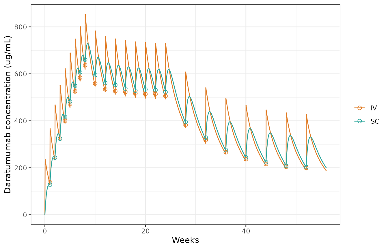
Replicates Figure 1A of Luo 2021: typical daratumumab profile after SC 1800 mg or IV 16 mg/kg (78.6 kg) on the approved monotherapy schedule. Lines are the model; points are the troughs digitised from the published figure.
typ_trough <- typ |>
  filter(abs(time - (round(time / 168) * 168 - 0.01)) < 1e-6) |>
  mutate(week = round(time / 168)) |>
  select(route, week, conc_model = Cc)

fig1a_cmp <- fig1a_trough |>
  left_join(typ_trough, by = c("route", "week")) |>
  mutate(pct_diff = 100 * (conc_model - conc_paper) / conc_paper)

fig1a_cmp |>
  group_by(route) |>
  summarise(
    n = n(),
    median_pct_diff = round(median(pct_diff), 1),
    max_abs_pct_diff = round(max(abs(pct_diff)), 1),
    .groups = "drop"
  ) |>
  dplyr::rename(
    Route = route, `Troughs compared` = n,
    `Median % diff` = median_pct_diff, `Max |% diff|` = max_abs_pct_diff
  ) |>
knitr::kable()| Route | Troughs compared | Median % diff | Max |% diff| |
|---|---|---|---|
| IV | 23 | -3.1 | 4.6 |
| SC | 23 | -0.7 | 2.9 |
peaks <- typ |>
  group_by(route) |>
  summarise(cmax = max(Cc), .groups = "drop")

stopifnot(
  # Every trough has a model counterpart (guards against a vacuous check).
  nrow(fig1a_cmp) == 46L,
  !anyNA(fig1a_cmp$conc_model),
  # Deterministic typical-value solve against an exactly digitised vector
  # figure: only digitisation and plotting-grid error separate the two.
  abs(median(fig1a_cmp$pct_diff)) < 5,
  max(abs(fig1a_cmp$pct_diff)) < 10,
  # Overall peak (week 8, cycle 3 day 1): IV 847 and SC 730 ug/mL in Figure 1A.
  abs(peaks$cmax[peaks$route == "IV"] / 847.4 - 1) < 0.05,
  abs(peaks$cmax[peaks$route == "SC"] / 730.3 - 1) < 0.05
)
The typical profiles reproduce Figure 1A throughout the 52 weeks for both routes, including the rise during weekly dosing, the plateau during every-2-week dosing and the decline once dosing moves to every 4 weeks. This confirms the parameter values, their units, the reference covariates and the time-decaying Vmax clock (time since the first dose).
Virtual cohort
The paper does not tabulate body weight (only its range), so the virtual cohort draws weight from a log-normal distribution with a median of 73 kg and a 22% CV, rejecting and redrawing values outside the observed 28.6-147.6 kg range. Albumin is normal with mean 39 g/L and SD 5.5 g/L, truncated to the observed 19-53 g/L; 58% have IgG myeloma and 43% are female (Table 2). The same covariate distribution is used for 200 SC and 200 IV monotherapy patients.
set.seed(20210614)
rxode2::rxSetSeed(20210614)
n_per_arm <- 200L

draw_wt <- function(n) {
  out <- numeric(0)
  while (length(out) < n) {
    x <- rlnorm(n, log(73), 0.22)
    out <- c(out, x[x >= 28.6 & x <= 147.6])
  }
  out[seq_len(n)]
}

make_cov <- function(route, id_offset) {
  data.frame(
    id = id_offset + seq_len(n_per_arm),
    route = route,
    WT = draw_wt(n_per_arm),
    ALB = pmin(53, pmax(19, rnorm(n_per_arm, 39, 5.5))),
    MM_NIGG = rbinom(n_per_arm, 1, 0.42),
    SEXF = rbinom(n_per_arm, 1, 0.43)
  )
}
cohort <- bind_rows(make_cov("SC", 0L), make_cov("IV", n_per_arm))

cohort_events <- bind_rows(
  lapply(seq_len(nrow(cohort)), function(i) {
    make_events(cohort$id[i], cohort$route[i], cohort$WT[i])
  }),
  tidyr::crossing(id = cohort$id, time = obs_times) |>
    mutate(amt = 0, evid = 0L, cmt = "central", rate = 0)
) |>
  left_join(cohort, by = "id") |>
  arrange(id, time, desc(evid))

sim <- rxode2::rxSolve(
  mod, cohort_events,
  keep = c("route", "WT"), returnType = "data.frame"
) |>
  filter(!is.na(Cc))
#> ℹ parameter labels from comments will be replaced by 'label()'
sim |>
  group_by(route, time) |>
  summarise(
    p05 = quantile(Cc, 0.05), p50 = median(Cc), p95 = quantile(Cc, 0.95),
    .groups = "drop"
  ) |>
  ggplot(aes(time / 168, p50, colour = route, fill = route)) +
  geom_ribbon(aes(ymin = p05, ymax = p95), alpha = 0.2, colour = NA) +
  geom_line() +
  scale_colour_manual(values = c(IV = "#E07B24", SC = "#2BA59B")) +
  scale_fill_manual(values = c(IV = "#E07B24", SC = "#2BA59B")) +
  labs(x = "Weeks", y = "Daratumumab concentration (ug/mL)", colour = NULL, fill = NULL) +
  theme_bw()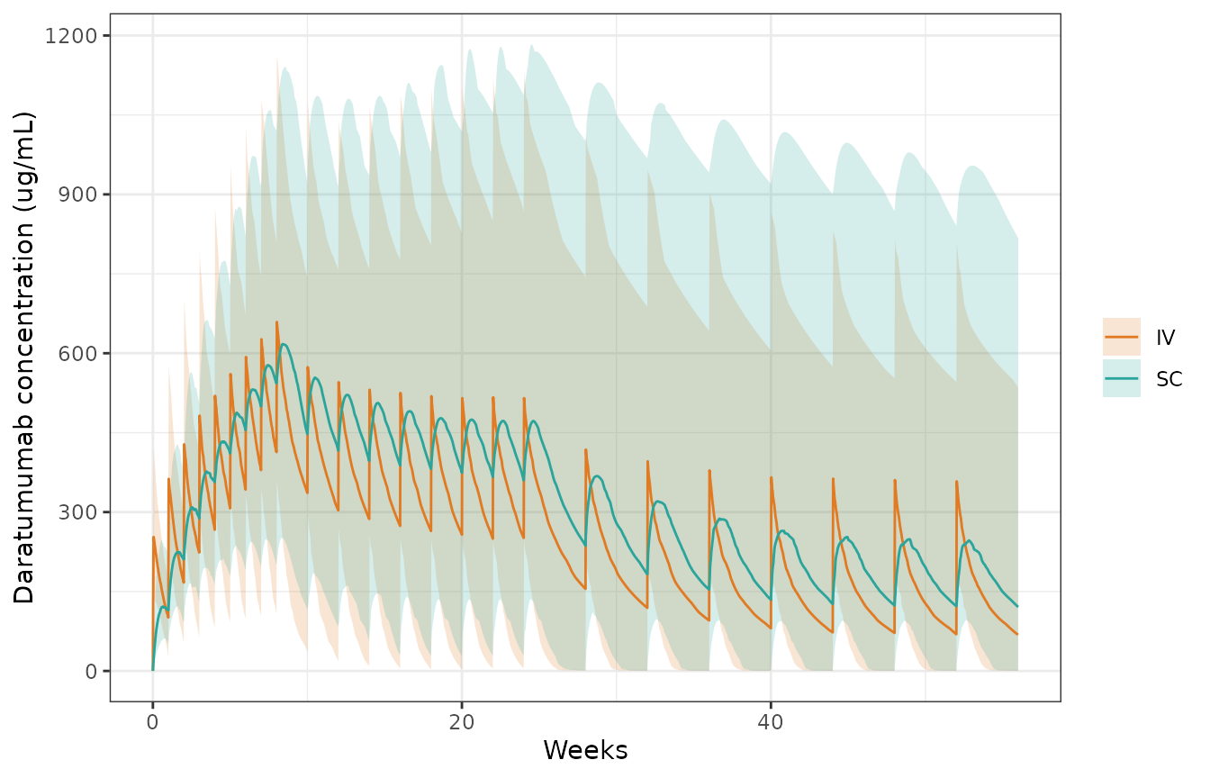
Simulated median and 5th-95th percentiles of daratumumab concentration for SC 1800 mg and IV 16 mg/kg monotherapy (200 virtual patients per route).
Maximum Ctrough (cycle 3 day 1) by body-weight subgroup
Luo 2021 (Results, ‘Influence of Body Weight’) reports simulated mean cycle 3 day 1 troughs (after 8 weekly doses) of 721 (SC) vs 432 ug/mL (IV) in patients of 65 kg or less and 472 (SC) vs 546 ug/mL (IV) above 85 kg, and calls the 65-85 kg subgroup comparable between routes.
ctrough_c3d1 <- sim |>
  filter(abs(time - (8 * 168 - 0.01)) < 1e-6) |>
  mutate(wt_group = cut(WT, c(0, 65, 85, Inf), labels = c("<=65 kg", ">65-85 kg", ">85 kg")))

wt_cmp <- ctrough_c3d1 |>
  group_by(route, wt_group) |>
  summarise(n = n(), mean_sim = mean(Cc), .groups = "drop") |>
  left_join(
    tibble(
      route = c("SC", "IV", "SC", "IV"),
      wt_group = factor(c("<=65 kg", "<=65 kg", ">85 kg", ">85 kg"), levels = c("<=65 kg", ">65-85 kg", ">85 kg")),
      mean_paper = c(721, 432, 472, 546)
    ),
    by = c("route", "wt_group")
  ) |>
  mutate(pct_diff = 100 * (mean_sim - mean_paper) / mean_paper)

wt_cmp |>
  mutate(across(c(mean_sim, pct_diff), \(x) round(x, 0))) |>
  dplyr::rename(
    Route = route, `Weight group` = wt_group, N = n,
    `Simulated mean (ug/mL)` = mean_sim, `Luo 2021 mean (ug/mL)` = mean_paper,
    `% diff` = pct_diff
  ) |>
knitr::kable()| Route | Weight group | N | Simulated mean (ug/mL) | Luo 2021 mean (ug/mL) | % diff |
|---|---|---|---|---|---|
| IV | <=65 kg | 59 | 374 | 432 | -13 |
| IV | >65-85 kg | 95 | 444 | NA | NA |
| IV | >85 kg | 46 | 547 | 546 | 0 |
| SC | <=65 kg | 66 | 681 | 721 | -5 |
| SC | >65-85 kg | 87 | 546 | NA | NA |
| SC | >85 kg | 47 | 443 | 472 | -6 |
wt_pct <- wt_cmp$pct_diff[!is.na(wt_cmp$pct_diff)]
sc_low <- wt_cmp$mean_sim[wt_cmp$route == "SC" & wt_cmp$wt_group == "<=65 kg"]
iv_low <- wt_cmp$mean_sim[wt_cmp$route == "IV" & wt_cmp$wt_group == "<=65 kg"]
stopifnot(
  length(wt_pct) == 4L,
  # Centre of the four published subgroup means.
  abs(median(wt_pct)) < 20,
  # The flat SC dose over-exposes light patients relative to weight-based IV
  # (paper: +67%); a mis-scaled dose or weight exponent collapses this gap.
  sc_low / iv_low > 1.3
)
Peak-to-trough ratio at cycle 3 day 1
The Results report a mean peak-to-trough ratio on cycle 3 day 1 of 1.2 for SC and 1.7 for IV. Here the ratio is the maximum concentration during the cycle 3 day 1 dosing interval (weeks 8-10) divided by the cycle 3 day 1 pre-dose trough.
ptr <- sim |>
  group_by(id, route) |>
  summarise(
    peak = max(Cc[time >= 8 * 168 & time <= 10 * 168]),
    trough = Cc[abs(time - (8 * 168 - 0.01)) < 1e-6],
    .groups = "drop"
  ) |>
  mutate(ratio = peak / trough)

ptr_summary <- ptr |>
  group_by(route) |>
  summarise(mean_ratio = mean(ratio), median_ratio = median(ratio), .groups = "drop") |>
  mutate(paper_mean = c(IV = 1.7, SC = 1.2)[route])

ptr_summary |>
  mutate(across(c(mean_ratio, median_ratio), \(x) round(x, 2))) |>
  dplyr::rename(
    Route = route, `Simulated mean` = mean_ratio, `Simulated median` = median_ratio,
    `Luo 2021 mean` = paper_mean
  ) |>
knitr::kable()| Route | Simulated mean | Simulated median | Luo 2021 mean |
|---|---|---|---|
| IV | 3.62 | 1.56 | 1.7 |
| SC | 1.19 | 1.14 | 1.2 |
stopifnot(
  abs(ptr_summary$median_ratio[ptr_summary$route == "SC"] / 1.2 - 1) < 0.15,
  ptr_summary$median_ratio[ptr_summary$route == "IV"] >
    ptr_summary$median_ratio[ptr_summary$route == "SC"] + 0.2
)
The SC ratio matches the published 1.2. The simulated IV mean is above the published 1.7 because a few simulated patients with high clearance have very low troughs; the median sits closer to the published value.
Half-life associated with linear elimination
Luo 2021 reports a geometric-mean half-life associated with linear
elimination of 20.4 days (22.4% CV) for monotherapy from post hoc
estimates. The paper does not define the calculation;
log(2) * V1 / CL reproduces it, while the terminal
(beta-phase) half-life of the linear two-compartment system is roughly
twice as long.
indiv <- sim |>
  group_by(id) |>
  slice(1) |>
  ungroup() |>
  mutate(
    k10 = cl / vc, k12 = q / vc, k21 = q / vp,
    beta = ((k10 + k12 + k21) - sqrt((k10 + k12 + k21)^2 - 4 * k10 * k21)) / 2,
    thalf_v1 = log(2) * vc / cl / 24,
    thalf_beta = log(2) / beta / 24
  )

gm <- function(x) exp(mean(log(x)))
thalf <- tibble(
  Quantity = c("log(2) * V1 / CL", "Terminal (beta) half-life, linear system"),
  `Simulated geometric mean (days)` = round(c(gm(indiv$thalf_v1), gm(indiv$thalf_beta)), 1),
  `Luo 2021 (days)` = c(20.4, NA)
)
knitr::kable(thalf)| Quantity | Simulated geometric mean (days) | Luo 2021 (days) |
|---|---|---|
| log(2) * V1 / CL | 20.5 | 20.4 |
| Terminal (beta) half-life, linear system | 46.1 | NA |
NCA of the first dose (PKNCA)
First-dose exposure over the first week (0-168 h) is summarised with PKNCA per route. Figure 6 of Luo 2021 gives the quartile boundaries of the first-dose Cmax pooled over SC and IV monotherapy patients (Q1 8.68-124, Q2 124-194, Q3 194-254, Q4 254-807 ug/mL), so the pooled median of 194 ug/mL is the published comparator.
conc_fd <- sim |>
  filter(time <= 168) |>
  select(id, treatment = route, time, Cc) |>
  filter(!is.na(Cc))

dose_fd <- cohort_events |>
  filter(evid == 1L, time == 0) |>
  select(id, treatment = route, time, amt)

conc_obj <- PKNCA::PKNCAconc(conc_fd, Cc ~ time | treatment + id, concu = "ug/mL", timeu = "h")
dose_obj <- PKNCA::PKNCAdose(dose_fd, amt ~ time | treatment + id, doseu = "mg")
intervals <- data.frame(start = 0, end = 168, cmax = TRUE, tmax = TRUE, auclast = TRUE)
nca_res <- PKNCA::pk.nca(PKNCA::PKNCAdata(conc_obj, dose_obj, intervals = intervals))

nca_res |>
  as.data.frame() |>
  group_by(treatment, PPTESTCD) |>
  summarise(median = signif(median(PPORRES), 3), .groups = "drop") |>
  tidyr::pivot_wider(names_from = PPTESTCD, values_from = median) |>
  dplyr::rename(
    Route = treatment, `Cmax (ug/mL)` = cmax, `Tmax (h)` = tmax,
    `AUC0-168 (h*ug/mL)` = auclast
  ) |>
knitr::kable(caption = "Median first-dose NCA by route (simulated).")| Route | AUC0-168 (h*ug/mL) | Cmax (ug/mL) | Tmax (h) |
|---|---|---|---|
| IV | 27900 | 253 | 8 |
| SC | 16500 | 125 | 122 |
cmax_pooled <- nca_res |>
  as.data.frame() |>
  filter(PPTESTCD == "cmax")

cmp <- nlmixr2lib::ncaComparisonTable(
  simulated = cmax_pooled |> select(PPTESTCD, PPORRES),
  reference = data.frame(cmax = 194),
  units = c(cmax = "ug/mL"),
  tolerance_pct = 20
)
knitr::kable(cmp, caption = "Pooled SC + IV first-dose Cmax, median (Luo 2021 Figure 6 quartile boundary).")| NCA parameter | Reference | Simulated | % diff |
|---|---|---|---|
| Cmax (ug/mL) | 194 | 184 | -4.9% |
q_sim <- quantile(cmax_pooled$PPORRES, c(0.25, 0.5, 0.75))
q_sim
#>      25%      50%      75%
#> 123.1138 184.4699 259.2743
stopifnot(
  nrow(cmax_pooled) == 2L * n_per_arm,
  abs(q_sim[[2]] / 194 - 1) < 0.2,
  # Interquartile boundaries (124 and 254 ug/mL) as an envelope check.
  abs(q_sim[[1]] / 124 - 1) < 0.25,
  abs(q_sim[[3]] / 254 - 1) < 0.25
)
Assumptions and deviations
-
Direction of the sex effect on V1. Table S1 prints
‘Sex on V1 = -0.105’ and its footnote defines SEXV1 as ‘1 for female and
1 [-] 0.105 for male’ (the minus sign is garbled to ‘to’ in the
supplement), so males have a 10.5% smaller V1 than females at equal
weight. The model follows the printed source (female reference,
1 + e_male_vc * (1 - SEXF)). This direction is opposite to the intravenous daratumumab model of Xu 2020 (Xu_2020_daratumumab, females 20.5% smaller V1), and no other open source (the FDA review reprints the table without the footnote) states it, so the label may have been swapped in the footnote. The effect is small (RSE 45.4%) and it does not change the reference-patient profile in Figure 1A. -
Vmax decay clock.
Vmax(t) = Vmax * exp(-KDES * t)withtthe time since the first dose, the form of the IV daratumumab model the SC model was built on. Figure 1A is reproduced with this clock. -
IIV. Table S1 reports IIV as %CV; variances are
log(CV^2 + 1). No covariances are reported, so the random effects are independent. -
Residual error. ‘Additive error term on the log
scale’ (34.8%) is encoded as log-normal error,
lnorm(expSd)withexpSd = 0.348. - Virtual cohort. Body weight (median 73 kg, 22% CV) and the albumin SD are not reported and are assumptions; the other covariate frequencies come from Table 2. The simulated cycle 3 day 1 troughs by weight subgroup fall within about 20% of the paper’s simulated means, which were computed from the individual estimates of the actual COLUMBA patients. Within a weight subgroup the mean depends on how weight, albumin and myeloma type are distributed, and the IV dose scales with weight while the SC dose does not, so an exact match is not expected from an assumed cohort.
- IV infusion duration. 7 h for the first infusion and 3.5 h thereafter, from the Introduction’s median infusion durations.
-
Half-life definition. The paper’s ‘half-life
associated with linear elimination’ is reproduced by
log(2) * V1 / CL; this definition is inferred, not stated. - Combination therapy (PLEIADES). The combination-therapy regimens use the same model (individual estimates were obtained by Bayesian post hoc estimation), so they are not simulated separately here.
- Exposure-response. The efficacy and safety analyses are graphical (exposure quartiles, logistic regression of adverse events on body weight) with no reported coefficients, so they are not part of the model.
- Errata. A literature check on 2026-09-28 found no erratum or correction for this article.