Bevacizumab biosimilar TAB008 mPBPK (Tsiros 2026)
Source:vignettes/articles/Tsiros_2026_bevacizumab_mpbpk.Rmd
Tsiros_2026_bevacizumab_mpbpk.RmdModel and source
- Citation: Tsiros P, Minadakis V, Sarimveis H. A physics-informed neural network approach for estimating population-level pharmacokinetic parameters from aggregated concentration data. J Pharmacokinet Pharmacodyn. 2026;53(2):11. doi:10.1007/s10928-026-10019-w. PMID 41699348. PMCID PMC12909361. Aggregated data from Wang J et al. Front Pharmacol. 2019;10:905. doi:10.3389/fphar.2019.00905 (TAB008 phase I). Model structure and fixed physiology from Cao Y, Balthasar JP, Jusko WJ. J Pharmacokinet Pharmacodyn. 2013;40(5):597-607. doi:10.1007/s10928-013-9332-2.
- Description: mPBPK. Minimal physiologically-based PK model (Cao 2013 second-generation structure; plasma, tight-tissue ISF, leaky-tissue ISF and lymph) for TAB008, a bevacizumab biosimilar, in healthy Chinese adult men after a single 1 mg/kg 90-min IV infusion. Fitted by distributional physics-informed neural networks (D-PINNs) to digitised mean and SD plasma concentrations; plasma clearance carries log-normal interindividual variability, physiological volumes scale with body weight, and the residual error is log-normal with its SD fixed at 0.1.
- Article: https://doi.org/10.1007/s10928-026-10019-w (open access, PMC12909361)
- Authors’ code and digitised data: https://github.com/ntua-unit-of-control-and-informatics/d-pinns-pharmacokinetics
Tsiros 2026 introduces distributional physics-informed neural networks (D-PINNs), which estimate population parameter distributions from published concentration means and variances instead of individual profiles. The paper has two case studies:
- A one-compartment IV-bolus model fitted to data simulated from hypothetical parameters (Vd 15 L, half-life 6 h). This is a demonstration of the method on an invented drug, so it is not packaged; the library already carries generic one-compartment structures.
- The second-generation minimal PBPK (mPBPK) model of Cao et al. (2013) fitted to aggregated plasma concentrations of TAB008, a bevacizumab biosimilar, from its phase I study (Wang 2019). This is the model packaged here.
Case study 2 was estimated twice, with D-PINNs and with a Stan MCMC
benchmark (Table 3). The packaged model carries the D-PINN estimates,
the method the paper proposes. The MCMC estimates are applied below
through ini() so that both columns of Table 3 and both
curves of Figure 12 can be reproduced.
Population
The data come from the PK part of a randomised, single-dose biosimilarity study of TAB008 against bevacizumab (Wang 2019): 49 healthy Chinese men aged 18 to 45 years, weighing 50 to 75 kg, each given 1 mg/kg TAB008 as a 90-minute IV infusion and sampled for up to 99 days. Individual data were not used: the authors digitised the published mean and SD serum concentrations (Tsiros 2026 Methods, “Monoclonal antibody data”). Because individual weights were also unavailable, body weight was drawn from Uniform(50, 75) kg during estimation, and this vignette does the same.
ui <- rxode2::rxode(readModelDb("Tsiros_2026_bevacizumab_mpbpk"))
#> ℹ parameter labels from comments will be replaced by 'label()'
str(ui$population)
#> List of 11
#>  $ species       : chr "human"
#>  $ n_subjects    : int 49
#>  $ n_studies     : int 1
#>  $ age_range     : chr "18-45 years"
#>  $ weight_range  : chr "50-75 kg"
#>  $ sex_female_pct: num 0
#>  $ race_ethnicity: chr "Chinese"
#>  $ disease_state : chr "Healthy volunteers"
#>  $ dose_range    : chr "1 mg/kg single IV infusion over 90 min"
#>  $ regions       : chr "China"
#>  $ notes         : chr "Tsiros 2026 Methods 'Monoclonal antibody data': the PK arm of the TAB008 phase I biosimilarity study (Wang 2019"| __truncated__
Source trace
| Equation / parameter | Value | Source location |
|---|---|---|
| Plasma ODE (in amounts) | d/dt(plasma) |
Eq. 28 |
| Tight-tissue ISF ODE | d/dt(tight) |
Eq. 29 |
| Leaky-tissue ISF ODE | d/dt(leaky) |
Eq. 30 |
| Lymph ODE | d/dt(lymph) |
Eq. 31 |
l1, l2
|
0.33 L, 0.67 L | Appendix C Eqs. 65-66 |
vtight, vleaky
|
0.65, 0.35 x V_ISF x Kp | Appendix C Eqs. 67-68 |
vblood |
0.073 x WT | Appendix C Eq. 69 |
visf |
0.15 x WT | Appendix C Eq. 70 |
vplasma |
V_blood x (1 - Hct) | Appendix C Eq. 71 |
vlymph |
V_blood | Appendix C Eq. 72 |
hct |
0.43 (fixed) | Appendix C text |
kp |
0.8 (fixed) | Appendix C text (native IgG1, Cao 2013) |
ltot |
3 L/day = 0.125 L/h (fixed) | Appendix C text |
sigmal |
0.2 (fixed) | Appendix C text |
sigma_tight |
0.8378 | Table 3, D-PINNs (sigma1) |
sigma_leaky |
0.7529 | Table 3, D-PINNs (sigma2) |
lcl |
log(0.010832) L/h | Table 3, D-PINNs: mean 0.0115, SD 0.0041, converted to the median (see below) |
etalcl |
0.119654 | Table 3, D-PINNs: log(1 + (0.0041/0.0115)^2) |
expSd |
0.1 (fixed) | Results, “Case study 2”; Eq. 14 |
| Dose | 1 mg/kg over 1.5 h | Methods, “Monoclonal antibody data” |
From the Table 3 moments to lcl and
etalcl
Table 3 reports mu_CLp and sigma_CLp. The
paper uses the same symbols in Table 1 for the arithmetic mean and SD of
a log-normal parameter (there, sigma_ke = 0.046 is the 40%
CV times the mean 0.116), and the authors’ Stan code reports exactly
these two quantities as mu_CL_normal = exp(mu + tau^2/2)
and tau_CL_normal. A log-normal with arithmetic mean
m and SD s has median
m / sqrt(1 + (s/m)^2) and log-scale variance
log(1 + (s/m)^2), which are what lcl and
etalcl hold.
lognormal_from_moments <- function(m, s) {
  cv2 <- (s / m)^2
  data.frame(
    mean = m, sd = s, cv_pct = 100 * sqrt(cv2),
    median = m / sqrt(1 + cv2), omega2 = log(1 + cv2)
  )
}
table3 <- data.frame(
  method = c("D-PINNs", "MCMC"),
  sigma_tight = c(0.8378, 0.8835),
  sigma_leaky = c(0.7529, 0.6657),
  mu_clp = c(0.0115, 0.0119),
  sigma_clp = c(0.0041, 0.0032)
)
derived <- cbind(
  table3[, c("method", "sigma_tight", "sigma_leaky")],
  lognormal_from_moments(table3$mu_clp, table3$sigma_clp)
)
knitr::kable(derived, digits = 6)| method | sigma_tight | sigma_leaky | mean | sd | cv_pct | median | omega2 |
|---|---|---|---|---|---|---|---|
| D-PINNs | 0.8378 | 0.7529 | 0.0115 | 0.0041 | 35.65217 | 0.010832 | 0.119655 |
| MCMC | 0.8835 | 0.6657 | 0.0119 | 0.0032 | 26.89076 | 0.011492 | 0.069816 |
Model with the MCMC estimates
mod_dpinn <- ui
# bquote() splices the numbers in, so ini() receives literals.
mod_mcmc <- eval(bquote(
  rxode2::ini(
    ui,
    lcl = .(log(derived$median[2])),
    sigma_tight = .(derived$sigma_tight[2]),
    sigma_leaky = .(derived$sigma_leaky[2]),
    etalcl ~ .(derived$omega2[2])
  )
))
#> ℹ change initial estimate of `lcl` to `-4.46612507449305`
#> ℹ change initial estimate of `sigma_tight` to `0.8835`
#> ℹ change initial estimate of `sigma_leaky` to `0.6657`
#> ℹ change initial estimate of `etalcl` to `0.0698163912567903`
stopifnot(abs(mod_mcmc$omega["etalcl", "etalcl"] / derived$omega2[2] - 1) < 1e-6)
mods <- list("D-PINNs" = mod_dpinn, "MCMC" = mod_mcmc)
Observed aggregated data
The mean and SD serum concentrations below are the values the authors
digitised from Wang 2019 and deposited with their code
(mPBPK/Data/preprocessed_mPBPK_data.csv). Time is from the
start of the infusion. The deposit holds 16 rows; the paper describes 15
measurements and Figure 12 plots the first 15 (to 2019.5 h). The 16th
row (2353.5 h, mean 0.207 mg/L with an SD of 0.867 mg/L) is shown here
but left out of the checks.
obs <- data.frame(
  time = c(0.75, 4, 25.5, 49.5, 97.5, 170.5, 244.5, 337.5, 505.5, 673.5,
           841.5, 1011.5, 1347.5, 1681.5, 2019.5, 2353.5),
  mean = c(8.350515, 19.25, 14.543104, 11.13885, 9.175316, 6.931276,
           6.370267, 5.41655, 3.815578, 2.75243, 2.064874, 1.509119,
           0.806089, 0.408646, 0.209887, 0.207163),
  sd = c(1.649485, 3.18, 2.726896, 2.199158, 1.974754, 1.413745, 1.357644,
         0.964937, 0.887048, 0.729692, 0.480044, 0.425186, 0.268409,
         0.165292, 0.117373, 0.867335)
)
knitr::kable(obs, digits = 3)| time | mean | sd |
|---|---|---|
| 0.75 | 8.351 | 1.649 |
| 4.00 | 19.250 | 3.180 |
| 25.50 | 14.543 | 2.727 |
| 49.50 | 11.139 | 2.199 |
| 97.50 | 9.175 | 1.975 |
| 170.50 | 6.931 | 1.414 |
| 244.50 | 6.370 | 1.358 |
| 337.50 | 5.417 | 0.965 |
| 505.50 | 3.816 | 0.887 |
| 673.50 | 2.752 | 0.730 |
| 841.50 | 2.065 | 0.480 |
| 1011.50 | 1.509 | 0.425 |
| 1347.50 | 0.806 | 0.268 |
| 1681.50 | 0.409 | 0.165 |
| 2019.50 | 0.210 | 0.117 |
| 2353.50 | 0.207 | 0.867 |
obs15 <- obs[obs$time < 2300, ]Virtual cohort and simulation
As in the paper’s Monte Carlo check (Results, “Case study 2”), each subject gets a body weight from Uniform(50, 75) kg, a 1 mg/kg dose infused over 1.5 h, and a clearance drawn from the estimated log-normal; a log-normal measurement error with SD 0.1 is then applied. The paper used 1000 subjects; 200 per parameter set are used here.
n_sub <- 200
obs_grid <- sort(unique(c(
  0, 0.25, 0.5, 0.75, 1, 1.25, 1.5, 2, 3, 4, 6, 8, 12, 24, 36, 48,
  seq(72, 2400, by = 24), obs$time
)))

make_events <- function(n, grid, seed) {
  set.seed(seed)
  wt <- stats::runif(n, 50, 75)
  dose <- data.frame(id = seq_len(n), time = 0, amt = wt, dur = 1.5,
                     evid = 1L, cmt = "plasma", WT = wt)
  obsr <- expand.grid(id = seq_len(n), time = grid)
  obsr$amt <- 0
  obsr$dur <- 0
  obsr$evid <- 0L
  obsr$cmt <- "plasma"
  obsr$WT <- wt[obsr$id]
  dplyr::arrange(rbind(dose, obsr), id, time, dplyr::desc(evid))
}

events <- make_events(n_sub, obs_grid, seed = 20260216)
rxode2::rxSetSeed(20260216)
sims <- dplyr::bind_rows(lapply(names(mods), function(nm) {
  s <- rxode2::rxSolve(mods[[nm]], events = events, returnType = "data.frame")
  s$method <- nm
  s
}))

# Measurement error exactly as Eq. 14 / Eq. 41: C = Ctrue * exp(eps).
set.seed(20260217)
sims$Cobs <- sims$Cc * exp(stats::rnorm(nrow(sims), 0, 0.1))
Figure 12: median and 95% prediction interval
Figure 12 plots the median and 95% prediction interval on a linear scale against time in hours; the same layout is used here.
band <- sims |>
  dplyr::filter(time >= 0.25) |>
  dplyr::group_by(method, time) |>
  dplyr::summarise(
    q025 = stats::quantile(Cobs, 0.025),
    q50 = stats::median(Cobs),
    q975 = stats::quantile(Cobs, 0.975),
    .groups = "drop"
  )

ggplot(dplyr::filter(band, time <= 2050), aes(time)) +
  geom_ribbon(aes(ymin = q025, ymax = q975, fill = method), alpha = 0.25) +
  geom_line(aes(y = q50, colour = method, linetype = method)) +
  geom_errorbar(data = obs15, inherit.aes = FALSE, width = 20,
                mapping = aes(x = time, ymin = mean - sd, ymax = mean + sd)) +
  geom_point(data = obs15, aes(x = time, y = mean), shape = 1, size = 2,
             inherit.aes = FALSE) +
  labs(x = "Time (h)", y = "TAB008 plasma concentration (mg/L)",
       colour = NULL, fill = NULL, linetype = NULL,
       caption = "Replicates Figure 12 of Tsiros 2026. Points: observed mean +/- SD.") +
  theme_bw()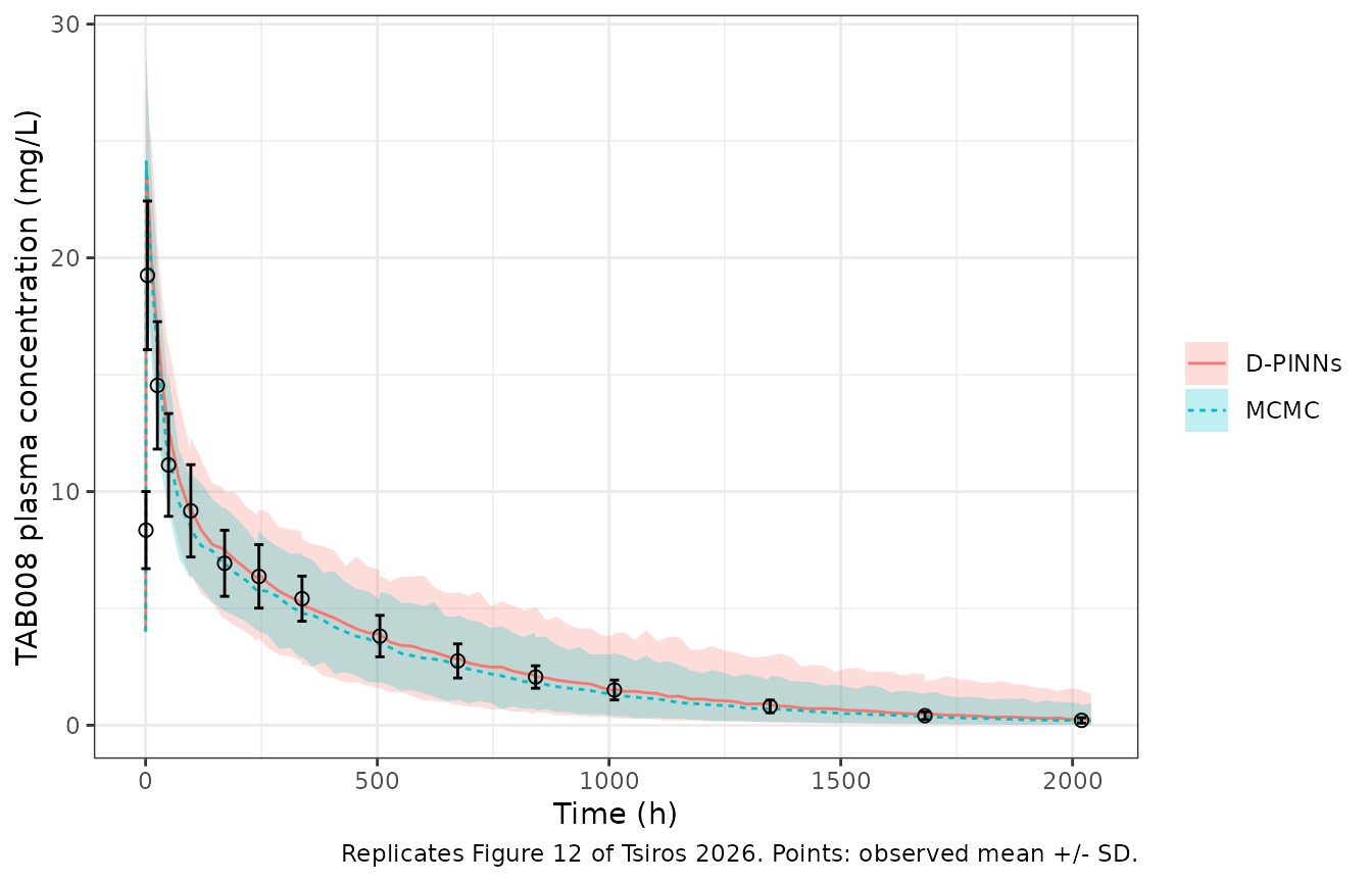
The D-PINN median read off Figure 12 (by eye, to about 0.5 mg/L) is close to 13, 9.2, 6.4, 3.9 and 1.5 mg/L at 49.5, 97.5, 244.5, 505.5 and 1011.5 h. The simulated median reproduces it:
fig12_dpinn <- data.frame(time = c(49.5, 97.5, 244.5, 505.5, 1011.5),
                          fig_median = c(13, 9.2, 6.4, 3.9, 1.5))
fig12_cmp <- band |>
  dplyr::filter(method == "D-PINNs") |>
  dplyr::inner_join(fig12_dpinn, by = "time") |>
  dplyr::mutate(pct_diff = 100 * (q50 / fig_median - 1))
fig12_cmp |>
  dplyr::select(time, fig_median, q50, pct_diff) |>
  dplyr::rename("Time (h)" = time, "Figure 12 median" = fig_median,
                "Simulated median" = q50, "Difference (%)" = pct_diff) |>
knitr::kable(digits = 2)| Time (h) | Figure 12 median | Simulated median | Difference (%) |
|---|---|---|---|
| 49.5 | 13.0 | 12.69 | -2.38 |
| 97.5 | 9.2 | 9.25 | 0.49 |
| 244.5 | 6.4 | 6.44 | 0.62 |
| 505.5 | 3.9 | 3.89 | -0.15 |
| 1011.5 | 1.5 | 1.55 | 3.39 |
The fitted quantities: simulated mean and SD at the sampling times
Both estimation methods fitted the model to the 15 observed means and SDs, so the simulated arithmetic mean and SD at those times are a direct check.
agg <- sims |>
  dplyr::filter(time %in% obs15$time) |>
  dplyr::group_by(method, time) |>
  dplyr::summarise(sim_mean = mean(Cobs), sim_sd = stats::sd(Cobs),
                   .groups = "drop") |>
  dplyr::inner_join(obs15, by = "time") |>
  dplyr::mutate(mean_pct_diff = 100 * (sim_mean / mean - 1),
                sd_pct_diff = 100 * (sim_sd / sd - 1))

agg |>
  dplyr::select(method, time, mean, sim_mean, mean_pct_diff, sd, sim_sd,
                sd_pct_diff) |>
  dplyr::rename("Time (h)" = time, "Observed mean" = mean,
                "Simulated mean" = sim_mean, "Mean diff (%)" = mean_pct_diff,
                "Observed SD" = sd, "Simulated SD" = sim_sd,
                "SD diff (%)" = sd_pct_diff) |>
knitr::kable(digits = 2)| method | Time (h) | Observed mean | Simulated mean | Mean diff (%) | Observed SD | Simulated SD | SD diff (%) |
|---|---|---|---|---|---|---|---|
| D-PINNs | 0.75 | 8.35 | 12.01 | 43.83 | 1.65 | 1.23 | -25.14 |
| D-PINNs | 4.00 | 19.25 | 23.19 | 20.49 | 3.18 | 2.23 | -29.76 |
| D-PINNs | 25.50 | 14.54 | 16.92 | 16.35 | 2.73 | 1.81 | -33.48 |
| D-PINNs | 49.50 | 11.14 | 12.80 | 14.91 | 2.20 | 1.67 | -23.99 |
| D-PINNs | 97.50 | 9.18 | 9.28 | 1.14 | 1.97 | 1.56 | -20.91 |
| D-PINNs | 170.50 | 6.93 | 7.40 | 6.70 | 1.41 | 1.37 | -3.24 |
| D-PINNs | 244.50 | 6.37 | 6.36 | -0.24 | 1.36 | 1.44 | 5.86 |
| D-PINNs | 337.50 | 5.42 | 5.24 | -3.26 | 0.96 | 1.52 | 57.72 |
| D-PINNs | 505.50 | 3.82 | 3.89 | 1.98 | 0.89 | 1.35 | 52.00 |
| D-PINNs | 673.50 | 2.75 | 2.96 | 7.55 | 0.73 | 1.29 | 77.00 |
| D-PINNs | 841.50 | 2.06 | 2.30 | 11.61 | 0.48 | 1.21 | 151.04 |
| D-PINNs | 1011.50 | 1.51 | 1.74 | 15.24 | 0.43 | 1.02 | 140.49 |
| D-PINNs | 1347.50 | 0.81 | 1.07 | 33.12 | 0.27 | 0.82 | 203.86 |
| D-PINNs | 1681.50 | 0.41 | 0.67 | 63.22 | 0.17 | 0.61 | 269.18 |
| D-PINNs | 2019.50 | 0.21 | 0.41 | 97.31 | 0.12 | 0.42 | 258.83 |
| MCMC | 0.75 | 8.35 | 11.91 | 42.66 | 1.65 | 1.22 | -25.93 |
| MCMC | 4.00 | 19.25 | 22.83 | 18.62 | 3.18 | 2.28 | -28.29 |
| MCMC | 25.50 | 14.54 | 16.02 | 10.16 | 2.73 | 1.86 | -31.70 |
| MCMC | 49.50 | 11.14 | 11.82 | 6.08 | 2.20 | 1.53 | -30.31 |
| MCMC | 97.50 | 9.18 | 8.45 | -7.92 | 1.97 | 1.16 | -41.08 |
| MCMC | 170.50 | 6.93 | 6.94 | 0.11 | 1.41 | 1.13 | -20.36 |
| MCMC | 244.50 | 6.37 | 5.87 | -7.81 | 1.36 | 1.06 | -21.66 |
| MCMC | 337.50 | 5.42 | 4.88 | -9.96 | 0.96 | 1.09 | 13.08 |
| MCMC | 505.50 | 3.82 | 3.55 | -6.91 | 0.89 | 1.08 | 21.28 |
| MCMC | 673.50 | 2.75 | 2.59 | -5.75 | 0.73 | 0.94 | 29.36 |
| MCMC | 841.50 | 2.06 | 1.94 | -6.05 | 0.48 | 0.83 | 73.77 |
| MCMC | 1011.50 | 1.51 | 1.45 | -4.17 | 0.43 | 0.71 | 66.94 |
| MCMC | 1347.50 | 0.81 | 0.81 | 0.90 | 0.27 | 0.51 | 90.62 |
| MCMC | 1681.50 | 0.41 | 0.48 | 16.85 | 0.17 | 0.37 | 123.24 |
| MCMC | 2019.50 | 0.21 | 0.27 | 28.67 | 0.12 | 0.25 | 109.15 |
mean_check <- agg |>
  dplyr::group_by(method) |>
  dplyr::summarise(median_abs_mean_diff = stats::median(abs(mean_pct_diff)),
                   q90_abs_mean_diff = stats::quantile(abs(mean_pct_diff), 0.9))
knitr::kable(mean_check, digits = 1)| method | median_abs_mean_diff | q90_abs_mean_diff |
|---|---|---|
| D-PINNs | 14.9 | 55.5 |
| MCMC | 7.8 | 24.7 |
# Centre only: the tails of the per-time differences are set by the 0.75 h
# point (mid-infusion) and by the log-normal skew at the late times, both of
# which the paper's own fit shares. Measured: about 15% (D-PINNs) and 8%
# (MCMC). A wrong unit on CL, a mis-scaled volume or a mistyped reflection
# coefficient moves the whole mean profile by tens of percent.
stopifnot(all(mean_check$median_abs_mean_diff < 25))
The simulated means follow the observed means for both parameter sets from 25 to about 1000 h. Two regions differ, in the same direction as the paper’s own Figure 12. At 0.75 h, halfway through the infusion, the observed mean of 8.4 mg/L is below the model’s ~12 mg/L; the published fit also passes above that point. After about 1000 h the D-PINN mean runs above the data, because its lower median clearance and larger clearance variability give a heavier upper tail; the simulated SD is likewise larger than the observed SD late on, which the paper reports (“the predicted variability was slightly overestimated at later time points”).
The two parameter sets give close median profiles. The D-PINN median clearance (0.0108 L/h) is about 6% lower than the MCMC one (0.0115 L/h), so the D-PINN median runs roughly 10% above the MCMC median over the first 1000 h, which is the small gap between the solid and dashed lines in Figure 12; the gap widens as the profiles decline further.
med_cmp <- band |>
  dplyr::filter(time >= 24, time <= 1011.5) |>
  dplyr::select(method, time, q50) |>
  tidyr::pivot_wider(names_from = method, values_from = q50) |>
  dplyr::mutate(ratio = `D-PINNs` / MCMC)
summary(med_cmp$ratio)
#>    Min. 1st Qu.  Median    Mean 3rd Qu.    Max.
#>   1.037   1.080   1.104   1.107   1.132   1.190
# Measured median ratio about 1.11.
stopifnot(abs(stats::median(med_cmp$ratio) - 1) < 0.2)
PKNCA validation
Typical-value profiles (no interindividual variability) for a 62.5 kg
subject, the midpoint of the weight range. All elimination is from
plasma at rate CL * Cp, so the plasma AUC from zero to
infinity must equal Dose / CL exactly; this checks the ODE
transcription independently of the fit.
grid_nca <- sort(unique(c(0, 10^seq(-2, log10(30000), length.out = 400))))
wt_ref <- 62.5
ev_typ <- dplyr::bind_rows(
  data.frame(id = 1L, time = 0, amt = wt_ref, dur = 1.5, evid = 1L,
             cmt = "plasma", WT = wt_ref),
  data.frame(id = 1L, time = grid_nca, amt = 0, dur = 0, evid = 0L,
             cmt = "plasma", WT = wt_ref)
)
typ <- dplyr::bind_rows(lapply(names(mods), function(nm) {
  s <- rxode2::rxSolve(rxode2::zeroRe(mods[[nm]]), events = ev_typ,
                       returnType = "data.frame", rtol = 1e-10, atol = 1e-12,
                       maxsteps = 1e6)
  if (is.null(s$id)) s$id <- 1L
  s$method <- nm
  s
}))
#> ℹ omega/sigma items treated as zero: 'etalcl'
#> ℹ omega/sigma items treated as zero: 'etalcl'
stopifnot(all(typ$Cc >= -1e-6 * max(typ$Cc)))

conc <- typ |>
  dplyr::filter(!is.na(Cc)) |>
  dplyr::mutate(Cc = pmax(Cc, 0)) |>
  dplyr::select(id, time, Cc, method)
dose_df <- data.frame(id = 1L, time = 0, amt = wt_ref,
                      method = names(mods))

conc_obj <- PKNCA::PKNCAconc(conc, Cc ~ time | method + id)
dose_obj <- PKNCA::PKNCAdose(dose_df, amt ~ time | method + id,
                             route = "intravascular", duration = 1.5)
intervals <- data.frame(start = 0, end = Inf, cmax = TRUE, tmax = TRUE,
                        aucinf.obs = TRUE, half.life = TRUE, cl.obs = TRUE,
                        vss.obs = TRUE)
nca <- PKNCA::pk.nca(PKNCA::PKNCAdata(conc_obj, dose_obj, intervals = intervals))
nca_tab <- as.data.frame(nca$result) |>
  dplyr::select(method, PPTESTCD, PPORRES) |>
  tidyr::pivot_wider(names_from = PPTESTCD, values_from = PPORRES)
nca_tab |>
  dplyr::select(method, cmax, tmax, aucinf.obs, half.life, cl.obs, vss.obs) |>
  dplyr::rename("Cmax (mg/L)" = cmax, "Tmax (h)" = tmax,
                "AUC0-inf (mg*h/L)" = aucinf.obs, "t1/2 (h)" = half.life,
                "CL (L/h)" = cl.obs, "Vss (L)" = vss.obs) |>
knitr::kable(digits = 4)| method | Cmax (mg/L) | Tmax (h) | AUC0-inf (mg*h/L) | t1/2 (h) | CL (L/h) | Vss (L) |
|---|---|---|---|---|---|---|
| D-PINNs | 23.7508 | 1.5542 | 5770.051 | 408.5277 | 0.0108 | 5.4074 |
| MCMC | 23.7064 | 1.5542 | 5438.773 | 396.7345 | 0.0115 | 5.6132 |
closed <- data.frame(method = names(mods),
                     auc_closed = wt_ref / derived$median)
chk <- dplyr::inner_join(nca_tab, closed, by = "method") |>
  dplyr::mutate(rel_err = aucinf.obs / auc_closed - 1)
knitr::kable(chk[, c("method", "aucinf.obs", "auc_closed", "rel_err")],
digits = 6)| method | aucinf.obs | auc_closed | rel_err |
|---|---|---|---|
| D-PINNs | 5770.051 | 5769.855 | 3.4e-05 |
| MCMC | 5438.773 | 5438.680 | 1.7e-05 |
# Same drawn parameters on both sides: the gap is quadrature plus
# extrapolation only, measured at about 3e-5 on the log-spaced grid.
stopifnot(all(abs(chk$rel_err) < 0.005))
The typical terminal half-life is about 17 days (408 h with the D-PINN estimates, 397 h with the MCMC estimates). The paper does not report non-compartmental parameters, so there is no published NCA table to compare against.
Assumptions and deviations
-
Table 3 moments.
mu_CLpandsigma_CLpare read as the arithmetic mean and SD of a log-normal clearance, consistent with Table 1 and with the quantities the authors’ Stan code reports. They are converted to the median (lcl) and log-scale variance (etalcl) above. Readingmu_CLpas the median instead would raise the typical clearance by 6% (D-PINNs) or 3.5% (MCMC). - Lymph flow is not weight-scaled. The Methods text lists L, L1 and L2 among the weight-dependent parameters, but Appendix C gives L as a constant 3 L/day and the authors’ code (both D-PINN and Stan) uses 0.125 L/h for every subject. The equations and code are followed.
- Blood-volume fraction. Appendix C prints 0.073 L/kg; the deposited D-PINN script uses 0.0733. The printed value is used.
-
Residual error. The paper’s log-normal measurement
error (
C = Ctrue * exp(eps), SD 0.1 held constant during estimation) is encoded aslnorm(expSd)withexpSdfixed at 0.1. -
Reflection coefficients have no IIV. The authors
deliberately estimated
sigma_tightandsigma_leakyas point values (Methods, “D-PINN implementation”), and the packaged model follows that. - Correlation terms. The D-PINN fit also estimates a correlation between the sampled plasma concentration and clearance. It is an internal device of the sampling scheme, not a model parameter, and is not carried.
-
Infusion timing. The dose is a zero-order infusion
over 1.5 h into the plasma amount, matching
Dose / T_infin Eq. 28. - Case study 1 (a hypothetical drug simulated from invented parameters) is not packaged.