Model and source
- Citation: Zuo P, Collins J, Okour M, Barth A, Shortino D, Yates P, Roberts G, Watson HA, Peppercorn A, Hossain M. Population pharmacokinetic/ pharmacodynamic analysis of intravenous zanamivir in healthy adults and hospitalized adult and pediatric subjects with influenza. Clin Transl Sci. 2020;13(1):157-168. doi:10.1111/cts.12697. Parameter estimates are the final-model column of Zuo 2020 Table 2; the creatinine-clearance equation is printed in the PopPK analysis Results paragraph; validation targets are Supplementary Tables S4 and S6.
- Description: Two-compartment population PK model for intravenous zanamivir with linear elimination, a piecewise-linear (hinge) creatinine-clearance effect on CL, a hospitalized-patient (suspected or confirmed influenza) effect on CL and on the magnitude of CL IIV, estimated allometric weight exponents on V1/V2 and Q, and a study effect on V1/V2, in healthy adults and hospitalized adult and pediatric subjects with influenza (Zuo 2020)
- Article: https://doi.org/10.1111/cts.12697 (open access; PMC6951463)
Population
The model was fitted to 5,273 serum zanamivir concentrations from 658 subjects pooled across eight studies of intravenous zanamivir: six phase I studies in 125 healthy adults (single doses of 100-1,200 mg and 300-600 mg twice daily) and two studies in hospitalized subjects with suspected or confirmed influenza – the phase II single-arm study NAI113678 (N = 180, including 54 pediatric subjects) and the phase III study NAI114373 (N = 353). Across the pooled data the median (range) age was 46 (0.6-101) years, body weight 72.0 (7.1-188.0) kg and creatinine clearance 91.8 (12.1-274.9) mL/min; 39% were female. Within the patient population 57% had renal impairment and 11% were younger than 18 years; 16 subjects were on renal replacement therapy and 10 on ECMO (Zuo 2020 Table 1 and Results). Renally impaired and pediatric patients received a renal-function- and weight-adjusted twice-daily maintenance dose (Table S1).
The same information is available programmatically via
readModelDb("Zuo_2020_zanamivir")()$population.
Source trace
Every ini() value carries an in-file source comment in
inst/modeldb/specificDrugs/Zuo_2020_zanamivir.R; the table
collects them.
| Equation / parameter | Value | Source location |
|---|---|---|
lcl (healthy, 70 kg, CrCL >= 97) |
log(6.82 L/h) | Table 2, final model |
lvc (V1, 70 kg) |
log(12.3 L) | Table 2, final model |
lq (70 kg) |
log(4.82 L/h) | Table 2, final model |
lvp (V2, 70 kg) |
log(6.52 L) | Table 2, final model |
lcrcl_hinge |
log(97.0 mL/min) | Table 2, ‘CL ~ CrCL (inflection point)’ |
e_crcl_cl |
0.00929 min/mL | Table 2, ‘CL ~ CrCL (slope)’ (final model; prose quotes the full-model 0.00923) |
e_flu_cl |
0.756 | Table 2, ‘CL ~ FLU’ |
e_flu_etalcl |
3.10 | Table 2, ‘IIV (CL) ~ FLU’ |
e_wt_vc_vp |
0.711 | Table 2, ‘V1/V2 ~ WT’ |
e_wt_q |
0.658 | Table 2, ‘Q ~ WT’ |
e_study_nai114346_vc_vp |
0.729 | Table 2, ‘V1/V2 ~ Study (NAI114346)’ |
etalcl |
0.034372 = log(1 + 0.187^2) | Table 2, IIV CL 18.7 CV% |
etalvc |
0.114313 = log(1 + 0.348^2) | Table 2, IIV V1 34.8 CV% |
propSd |
0.262 | Table 2, proportional error 26.2 CV% |
addSd |
0.0269 ug/mL | Table 2, additive error SD |
CrCL hinge 1 + (CrCL - 97) x slope below 97, 1
above |
n/a | Results, PopPK analysis paragraph 1 |
| Two-compartment, IV infusion, first-order elimination | n/a | Results and Discussion |
| 30-minute infusion (used in the simulations below) | n/a | Table S2: end of infusion sampled at 0.5 h |
Typical-value checks against the paper’s own numbers
mod <- readModelDb("Zuo_2020_zanamivir")
ini_df <- rxode2::rxode(mod)$iniDf
#> ℹ parameter labels from comments will be replaced by 'label()'
#> Warning: some etas defaulted to non-mu referenced, possible parsing error: etalcl
#> as a work-around try putting the mu-referenced expression on a simple line
th <- setNames(ini_df$est, ini_df$name)

cl_healthy <- exp(th[["lcl"]])
cl_patient <- cl_healthy * th[["e_flu_cl"]]
vss_70 <- exp(th[["lvc"]]) + exp(th[["lvp"]])

typical <- tibble::tribble(
  ~quantity, ~model, ~paper,
  "CL, healthy 70 kg (L/h)", cl_healthy, 6.82,
  "CL, influenza patient 70 kg (L/h)", cl_patient, 5.16,
  "Vss = V1 + V2 at 70 kg (L)", vss_70, 18.8
)
knitr::kable(typical, digits = 3, caption = "Results paragraph 3 and Discussion.")| quantity | model | paper |
|---|---|---|
| CL, healthy 70 kg (L/h) | 6.820 | 6.82 |
| CL, influenza patient 70 kg (L/h) | 5.156 | 5.16 |
| Vss = V1 + V2 at 70 kg (L) | 18.820 | 18.80 |
The creatinine-clearance equation
The Results print the CrCL effect as
1 + (CrCL - 97) x slope below 97 mL/min. The next paragraph
then quotes clearance reductions of 26-54% for mild impairment (CrCL 50
to <80), 54-72% moderate, 72-86% severe and >86% end-stage. Those
four ranges are reproduced exactly by CrCL x 0.00929
(e.g. 80 x 0.00929 = 0.74, 15 x 0.00929 = 0.14), not by the printed
equation (which gives 16-44% for mild impairment). The model file
follows the printed equation, and Supplementary Table S6 – the paper’s
own simulation output – settles which one the fit used: the
geometric-mean steady-state AUC0-tau after 300 mg twice daily in adults
gives the clearance the authors simulated with,
CL = 300 / AUC.
f_printed <- function(crcl) {
  1 + th[["e_crcl_cl"]] * (pmin(crcl, exp(th[["lcrcl_hinge"]])) - exp(th[["lcrcl_hinge"]]))
}
f_prose <- function(crcl) pmin(crcl * th[["e_crcl_cl"]], 1)

s6 <- tibble::tribble(
  ~renal, ~crcl_mid, ~auc_s6,
  "50 to <80", 65, 80.92,
  "30 to <50", 40, 122.4,
  "15 to <30", 22.5, 186.50
) |>
  mutate(
    cl_s6 = 300 / auc_s6,
    ratio_s6 = cl_s6 / (300 / 58.45),
    ratio_printed = f_printed(crcl_mid),
    ratio_prose = f_prose(crcl_mid)
  )
knitr::kable(
  s6,
  digits = 3,
  caption = paste(
    "CL ratio relative to CrCL >= 80, from Table S6 AUC0-tau (300 mg BID adults),",
    "against the printed equation and the prose reading at each band midpoint."
  )
)| renal | crcl_mid | auc_s6 | cl_s6 | ratio_s6 | ratio_printed | ratio_prose |
|---|---|---|---|---|---|---|
| 50 to <80 | 65.0 | 80.92 | 3.707 | 0.722 | 0.703 | 0.604 |
| 30 to <50 | 40.0 | 122.40 | 2.451 | 0.478 | 0.470 | 0.372 |
| 15 to <30 | 22.5 | 186.50 | 1.609 | 0.313 | 0.308 | 0.209 |
Scaling of CL variability in patients
Table 2 reports a 3.10 ‘IIV (CL) ~ FLU’ factor without saying whether it scales the random effect (standard deviation) or its variance. The two readings give very different patient CL variability, and the post hoc CL in adult patients with CrCL >= 80 mL/min in Supplementary Table S4 has a geometric CV of 64%:
omega2_cl <- th[["etalcl"]]
cv_sd_scaled <- sqrt(exp(omega2_cl * th[["e_flu_etalcl"]]^2) - 1)
cv_var_scaled <- sqrt(exp(omega2_cl * th[["e_flu_etalcl"]]) - 1)
knitr::kable(
  tibble::tibble(
    reading = c("eta multiplied by 3.10 (used)", "variance multiplied by 3.10"),
    `patient CL CV` = c(cv_sd_scaled, cv_var_scaled),
    `Table S4 post hoc CV` = 0.64
  ),
  digits = 2
)| reading | patient CL CV | Table S4 post hoc CV |
|---|---|---|
| eta multiplied by 3.10 (used) | 0.63 | 0.64 |
| variance multiplied by 3.10 | 0.34 | 0.64 |
Scaling the random effect (the usual NONMEM
ETA(1) * THETA idiom) gives 63%, in line with the 64% post
hoc spread (which shrinkage can only reduce); scaling the variance gives
33%. The model uses the former.
Terminal half-life
thalf <- function(crcl, wt = 70) {
  cl <- cl_patient * f_printed(crcl)
  vc <- exp(th[["lvc"]]) * (wt / 70)^th[["e_wt_vc_vp"]]
  vp <- exp(th[["lvp"]]) * (wt / 70)^th[["e_wt_vc_vp"]]
  q <- exp(th[["lq"]]) * (wt / 70)^th[["e_wt_q"]]
  k10 <- cl / vc
  k12 <- q / vc
  k21 <- q / vp
  s <- k10 + k12 + k21
  beta <- (s - sqrt(s^2 - 4 * k10 * k21)) / 2
  log(2) / beta
}
hl <- tibble::tibble(
  group = c("adult patient, CrCL >= 97", "adult patient, CrCL 10 (end-stage)"),
  model = c(thalf(120), thalf(10)),
  paper = c(3.2, 8.93)
)
knitr::kable(hl, digits = 2, caption = "Results: t1/2 3.2 h (normal renal function) and 8.93 h (end-stage), Table S5.")| group | model | paper |
|---|---|---|
| adult patient, CrCL >= 97 | 2.94 | 3.20 |
| adult patient, CrCL 10 (end-stage) | 13.53 | 8.93 |
The end-stage value depends strongly on the CrCL chosen within the <15 mL/min band (the paper’s six end-stage subjects are not described further); the typical value at CrCL 10 mL/min is shown for orientation only.
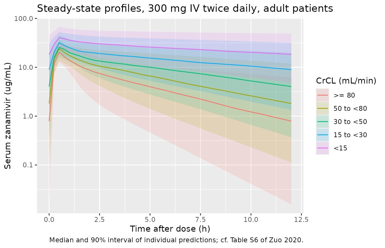
Virtual cohort and simulation: 300 mg twice daily at steady state
Supplementary Table S6 summarizes 1,000 simulations of 300 mg twice
daily in adult influenza patients by renal-function band. The virtual
cohort below uses 150 adult patients per band
(DIS_HEALTHY = 0, not in study NAI114346), body weight
log-normal around 72 kg, and CrCL uniform within each band. Doses are
30-minute infusions every 12 hours for 5 days; the last interval (96-108
h) is analysed.
set.seed(2020)
bands <- tibble::tribble(
  ~renal, ~crcl_lo, ~crcl_hi,
  ">= 80", 80, 160,
  "50 to <80", 50, 80,
  "30 to <50", 30, 50,
  "15 to <30", 15, 30,
  "<15", 5, 15
)
n_per <- 150L

subjects <- bands |>
  mutate(band_id = row_number()) |>
  tidyr::uncount(n_per) |>
  mutate(
    id = row_number(),
    CRCL = runif(n(), crcl_lo, crcl_hi),
    WT = pmin(pmax(exp(rnorm(n(), log(72), 0.25)), 40), 150),
    DIS_HEALTHY = 0L,
    STUDY_NAI114346 = 0L
  )

dose_times <- seq(0, 108, by = 12)
obs_times <- sort(unique(c(seq(96, 108, by = 0.25), 96.5)))

dosing <- subjects |>
  tidyr::crossing(time = dose_times) |>
  mutate(evid = 1L, amt = 300, rate = 600, cmt = "central")
obs <- subjects |>
  tidyr::crossing(time = obs_times) |>
  mutate(evid = 0L, amt = 0, rate = 0, cmt = "central")
events <- bind_rows(dosing, obs) |>
  arrange(id, time, desc(evid)) |>
  select(id, time, evid, amt, rate, cmt, CRCL, WT, DIS_HEALTHY, STUDY_NAI114346, renal)
sim <- rxode2::rxSolve(mod, events = events, keep = "renal", returnType = "data.frame")
#> ℹ parameter labels from comments will be replaced by 'label()'
#> Warning: some etas defaulted to non-mu referenced, possible parsing error: etalcl
#> as a work-around try putting the mu-referenced expression on a simple line
sim$renal <- factor(sim$renal, levels = bands$renal)
sim |>
  group_by(renal, time) |>
  summarise(
    Q05 = quantile(Cc, 0.05),
    Q50 = median(Cc),
    Q95 = quantile(Cc, 0.95),
    .groups = "drop"
  ) |>
  ggplot(aes(time - 96, Q50, colour = renal, fill = renal)) +
  geom_ribbon(aes(ymin = Q05, ymax = Q95), alpha = 0.15, colour = NA) +
  geom_line() +
  scale_y_log10() +
  labs(
    x = "Time after dose (h)", y = "Serum zanamivir (ug/mL)",
    colour = "CrCL (mL/min)", fill = "CrCL (mL/min)",
    title = "Steady-state profiles, 300 mg IV twice daily, adult patients",
    caption = "Median and 90% interval of individual predictions; cf. Table S6 of Zuo 2020."
  )
PKNCA validation against Table S6
sim_nca <- sim |>
  filter(!is.na(Cc)) |>
  select(id, time, Cc, renal)

conc_obj <- PKNCA::PKNCAconc(sim_nca, Cc ~ time | renal + id)
dose_df <- events |>
  filter(evid == 1) |>
  select(id, time, amt, renal)
dose_obj <- PKNCA::PKNCAdose(dose_df, amt ~ time | renal + id)

intervals <- data.frame(
  start = 96, end = 108,
  cmax = TRUE, auclast = TRUE, cmin = TRUE
)
nca_res <- PKNCA::pk.nca(PKNCA::PKNCAdata(conc_obj, dose_obj, intervals = intervals))
Table S6 values are geometric means across the simulated population
(adults, 300 mg twice daily); cmin over the dosing interval
is the trough C-tau.
published <- tibble::tribble(
  ~renal, ~auclast, ~cmax, ~cmin,
  ">= 80", 58.45, 20.69, 0.72,
  "50 to <80", 80.92, 23.17, 1.61,
  "30 to <50", 122.4, 28.69, 3.60,
  "15 to <30", 186.50, 35.52, 7.79,
  "<15", 249.90, 42.46, 12.38
)

cmp <- nlmixr2lib::ncaComparisonTable(
  simulated = nca_res,
  reference = published,
  by = "renal",
  units = c(auclast = "h*ug/mL", cmax = "ug/mL", cmin = "ug/mL"),
  tolerance_pct = 20
)
knitr::kable(
  cmp,
  caption = "Simulated vs. Table S6 (300 mg BID, adults). * differs from reference by >20%."
)| NCA parameter | renal | Reference | Simulated | % diff |
|---|---|---|---|---|
| Cmax (ug/mL) | >= 80 | 20.7 | 20.3 | -2.1% |
| Cmax (ug/mL) | 50 to <80 | 23.2 | 24.1 | +3.9% |
| Cmax (ug/mL) | 30 to <50 | 28.7 | 25.7 | -10.5% |
| Cmax (ug/mL) | 15 to <30 | 35.5 | 31.9 | -10.1% |
| Cmax (ug/mL) | <15 | 42.5 | 40.5 | -4.7% |
| Cmin (ug/mL) | >= 80 | 0.72 | 0.79 | +9.8% |
| Cmin (ug/mL) | 50 to <80 | 1.61 | 1.82 | +12.7% |
| Cmin (ug/mL) | 30 to <50 | 3.6 | 4.04 | +12.1% |
| Cmin (ug/mL) | 15 to <30 | 7.79 | 8.97 | +15.2% |
| Cmin (ug/mL) | <15 | 12.4 | 18.3 | +47.9%* |
| AUClast (h*ug/mL) | >= 80 | 58.4 | 56.4 | -3.5% |
| AUClast (h*ug/mL) | 50 to <80 | 80.9 | 88.7 | +9.6% |
| AUClast (h*ug/mL) | 30 to <50 | 122 | 120 | -2.0% |
| AUClast (h*ug/mL) | 15 to <30 | 186 | 181 | -2.9% |
| AUClast (h*ug/mL) | <15 | 250 | 304 | +21.5%* |
sim_gm <- as.data.frame(nca_res) |>
  filter(PPTESTCD %in% c("auclast", "cmax")) |>
  group_by(renal, PPTESTCD) |>
  summarise(sim = exp(mean(log(PPORRES))), .groups = "drop")
chk <- published |>
  select(renal, auclast, cmax) |>
  tidyr::pivot_longer(-renal, names_to = "PPTESTCD", values_to = "ref") |>
  inner_join(sim_gm, by = c("renal", "PPTESTCD")) |>
  mutate(pct_diff = 100 * (sim / ref - 1))
knitr::kable(chk, digits = 1)| renal | PPTESTCD | ref | sim | pct_diff |
|---|---|---|---|---|
| >= 80 | auclast | 58.5 | 55.5 | -5.0 |
| >= 80 | cmax | 20.7 | 20.5 | -0.8 |
| 50 to <80 | auclast | 80.9 | 84.8 | 4.9 |
| 50 to <80 | cmax | 23.2 | 23.3 | 0.8 |
| 30 to <50 | auclast | 122.4 | 121.0 | -1.2 |
| 30 to <50 | cmax | 28.7 | 25.9 | -9.6 |
| 15 to <30 | auclast | 186.5 | 186.9 | 0.2 |
| 15 to <30 | cmax | 35.5 | 31.6 | -11.1 |
| <15 | auclast | 249.9 | 294.5 | 17.8 |
| <15 | cmax | 42.5 | 40.1 | -5.6 |
# Assert on the centre of each band; the lowest band's CrCL distribution is
# not published, so it is excluded from the AUC check.
chk_core <- chk |> filter(!(renal == "<15" & PPTESTCD == "auclast"))
stopifnot(
  abs(median(chk_core$pct_diff)) < 10,
  all(abs(chk_core$pct_diff) < 25)
)
AUC0-tau and Cmax reproduce Table S6 in every band where the CrCL range is bounded. The end-stage band depends on the unpublished CrCL distribution below 15 mL/min, and the trough is the most sensitive to the assumed weight and CrCL distributions, so both are shown but not asserted tightly.
Assumptions and deviations
-
CrCL equation. The printed equation
1 + (CrCL - 97) x 0.00929is used. The Results prose’s percentage reductions correspond toCrCL x 0.00929; Supplementary Table S6 (the paper’s own simulation) agrees with the printed equation, so the prose percentages are treated as a paper-side slip. The prose also quotes the full-model slope (0.00923); the final-model value (0.00929) from Table 2 is used. -
IIV scaling in patients.
IIV (CL) ~ FLU = 3.10is implemented as a multiplier on the CL random effect (standard-deviation scale), which reproduces the Table S4 post hoc CL variability; see the check above. -
Healthy-participant indicator. The source flag
FLU(1 = hospitalized suspected or confirmed influenza patient) is encoded with the canonicalDIS_HEALTHYasFLU = 1 - DIS_HEALTHY. The paper’s reference individual is healthy (Figure 1). - CrCL units. The source CrCL column is Cockcroft-Gault in mL/min for subjects aged 13 years or older and Schwartz in mL/min/1.73 m^2 for younger children (Table S4-S6 footnotes); the model uses the value as supplied, with no conversion.
- Infusion duration. Not stated for every study; 30 minutes is inferred from the end-of-infusion samples at 0.5 h in Table S2 and used in the simulations.
-
Dropped covariates. RRT and ECMO effects on CL were
in the full model but not the final model; they are recorded in
covariatesDataExcluded. - Not extracted. The exposure-response analyses (Cox proportional-hazards models of time to clinical and virologic response, and viral-load plots) found no significant exposure effect and report no exposure coefficients, so there is no PD model to encode. The target-attainment percentages of Table 3 depend on the full simulated patient covariate distribution, which is not published, and are not reproduced.
- Virtual cohort. Body weight and within-band CrCL distributions are assumptions (log-normal around 72 kg; uniform within band).