Serotonergic thermoregulation in mice: harmaline + 5-MeO-DMT (Jiang 2016)
Source:vignettes/articles/Jiang_2016_harmaline_meodmt_mouse.Rmd
Jiang_2016_harmaline_meodmt_mouse.RmdThe model
Jiang XL, Shen HW, Mager DE, Schmidt S, Yu AM. Development of a mechanism-based pharmacokinetic/pharmacodynamic model to characterize the thermoregulatory effects of serotonergic drugs in mice. Acta Pharm Sin B. 2016;6(5):492-503. doi:10.1016/j.apsb.2016.07.007
The paper builds one integrated PK/PD model (its Fig. 1) linking the pharmacokinetics of the monoamine oxidase-A inhibitor harmaline and the 5-HT receptor agonist 5-MeO-DMT to core body temperature (CBT) in mice. Three things are happening at once:
- a pharmacokinetic interaction – harmaline competitively inhibits two of the three routes that clear 5-MeO-DMT, so harmaline raises 5-MeO-DMT exposure;
- a pharmacodynamic interaction – harmaline lowers the 5-MeO-DMT concentration producing half-maximal thermogenesis roughly 4-fold;
- a genotype effect – CYP2D6-humanized transgenic mice clear harmaline faster than wild-type mice, which blunts harmaline’s hypothermia.
mod <- rxode2::rxode(readModelDb("Jiang_2016_harmaline_meodmt_mouse"))
mod$state
#>  [1] "depot_harmaline"       "central_harmaline"     "peripheral1_harmaline"
#>  [4] "depot_meodmt"          "central_meodmt"        "peripheral1_meodmt"
#>  [7] "stress"                "transit1"              "transit2"
#> [10] "transit3"              "temp"
Population
pop <- mod$population
knitr::kable(
  data.frame(Field = names(pop), Value = unlist(lapply(pop, as.character))),
  row.names = FALSE
)| Field | Value |
|---|---|
| species | mouse (male FVB/N wild-type and Tg-CYP2D6 humanized) |
| n_per_group | 26 per genotype for the saline / baseline arms (Fig. 2); 14 per genotype for the single-drug arms (Fig. 3); 11 wild-type and 12 Tg-CYP2D6 for the combination arms (Figs. 4, 6); 4-14 per genotype for the external validation arms (Fig. 5) |
| n_studies | 1 |
| weight_range | 25-35 g |
| sex_female_pct | 0 |
| disease_state | healthy; drug-induced thermoregulatory perturbation |
| dose_range | harmaline 2-15 mg/kg i.p. and 5-MeO-DMT 2-20 mg/kg i.p., alone and in combination |
| regions | United States (University at Buffalo, SUNY) |
| notes | Telemetric core body temperature (Physiotel TA10TA-F20) sampled 10 times per minute and averaged over 5 or 10 min for modelling; ambient temperature 20 +/- 2 degC, 12 h light/dark cycle, observation window 10:30 a.m. to 3:30 p.m. Fitted in ADAPT V by naive-pooled maximum likelihood, so the model carries typical values only and no inter-individual variability. |
Male FVB/N wild-type and Tg-CYP2D6 mice, 25-35 g, dosed intraperitoneally. Core body temperature was recorded by implanted telemetry at 10 samples per minute and averaged over 5- or 10-minute bins for modelling. The fit was a naive-pooled maximum-likelihood analysis in ADAPT V, so the model carries typical values only – there is no inter-individual variability to simulate and every check below is deterministic.
Source trace
Every value in ini() comes from the locations below.
| Quantity | Source |
|---|---|
| Harmaline PK: ka-H, VC-H, VP-H, CLD-H, CLother-H, CLCYP2D6-H, FH | Methods 2.4, p. 494 (values carried over from the companion PK study, ref. 27, and held fixed here) |
| 5-MeO-DMT PK: ka-M, VC-M, VP-M, CLD-M, FM | Methods 2.4, p. 494 |
| 5-MeO-DMT elimination: Vmax and Km for MAO-A, other murine, O-demethylation | Methods 2.4, p. 494 |
| fmCYP2D6(D)-M = 30.1% | Methods 2.4, p. 494; the multiplicative form Vmax(D)-M x (1 + fm) is printed inside the Fig. 1 schematic |
| Ki(M)-H = 0.048 umol/L | Methods 2.4, p. 494 (literature value, ref. 32) |
| Ki(D)-H = 7.13 umol/L | Methods 2.4, p. 495 (from the upstream PK model fitting) |
| Competitive (on Km) form of both inhibition terms | Fig. 1: both Ki arrows terminate in an inhibition bar on the Km label, not the Vmax label |
| Baseline CBT equation | Eq. (1) |
| Indirect-response turnover with adaptive feedback | Eq. (2), closed at time zero by Eq. (3) |
| Handling/injection stress signal | Eq. (4) |
| Harmaline stimulation of heat loss (5-HT1A) | Eq. (5) |
| 5-MeO-DMT transduction chain (3 transit compartments) | Eqs. (6)-(8) |
| Final thermoregulatory ODE | Eq. (9) |
| Residual-error structure | Eq. (10) gives the form; no sigma value is printed anywhere in the paper |
| All PD parameter values and their CV% | Table 1 |
Units
Every published volume, clearance and Vmax is weight-normalised, so the whole system is per kg body weight and compartment amounts are umol/kg.
| Term | Units | Checks |
|---|---|---|
| central_harmaline | umol/kg | amount per kg |
| Cc_harmaline = central_harmaline / vc_harmaline | umol/L | (umol/kg) / (L/kg) |
| cl_harmaline * Cc_harmaline | umol/min/kg | (L/min/kg) x (umol/L) |
| elim_meodmt | umol/min/kg | Vmax already umol/min/kg; the MM fraction is unitless |
| sH = ks_harmaline * Cc_harmaline | unitless | (L/umol) x (umol/L) |
| kin = kout * rbase | degC/min | (1/min) x degC |
| kin * (tempBasal / temp) | degC/min | feedback ratio is unitless |
| kout * (1 + sH) * temp | degC/min | (1/min) x degC |
Note the one unit inconsistency in the source: CLother-H
and CLCYP2D6-H are printed as “L/min” while every other
volume and clearance in the same paragraph carries “/kg”. They must be
L/min/kg for the model to be dimensionally consistent,
and the check under “Harmaline pharmacokinetics” below confirms this
against the paper’s own simulated concentrations.
Setting up simulations
Doses are published in mg/kg; the model works in umol/kg. The two molecular weights are chemical constants and are not taken from the paper.
MW_HARMALINE <- 214.26 # g/mol, harmaline free base
MW_MEODMT <- 218.30 # g/mol, 5-MeO-DMT free base

# One arm of the experiment. `inj_extra` adds a second handling/injection event
# at `t_second` even when nothing pharmacological is given (the vehicle arms).
simulate_arm <- function(label, dose_harmaline = 0, dose_meodmt = 0, tg = 0,
                         t_second = 15, inj_extra = FALSE, tmax = 240,
                         dt = 0.5) {
  inj_times <- numeric(0)
  ev <- rxode2::et(seq(0, tmax, by = dt), cmt = "temp")

  if (dose_harmaline > 0) {
    ev <- rxode2::et(
      ev,
      amt = dose_harmaline / MW_HARMALINE * 1000,
      cmt = "depot_harmaline", time = 0
    )
    inj_times <- c(inj_times, 0)
  }
  if (dose_meodmt > 0) {
    ev <- rxode2::et(
      ev,
      amt = dose_meodmt / MW_MEODMT * 1000,
      cmt = "depot_meodmt", time = t_second
    )
    inj_times <- c(inj_times, t_second)
  }
  if (inj_extra) inj_times <- c(inj_times, t_second)

  # One unit into `stress` per handling event; the model's f(stress) scales it
  # to the published magnitude S0 = 0.265.
  for (tt in sort(unique(inj_times))) {
    ev <- rxode2::et(ev, amt = 1, cmt = "stress", time = tt)
  }

  d <- as.data.frame(ev)
  d$CYP2D6_TG <- tg
  # kS-H switches on the handling burden, not on what was injected.
  d$INJ_REPEAT <- as.integer(length(unique(inj_times)) > 1)
  # SC50-M switches on whether harmaline was actually present.
  d$CONMED_HARMALINE <- as.integer(dose_harmaline > 0 && dose_meodmt > 0)
  d$DOSE_HARMALINE_MGKG <- dose_harmaline

  out <- rxode2::rxSolve(mod, d, returnType = "data.frame")
  out$arm <- label
  out$genotype <- ifelse(tg == 1, "Tg-CYP2D6", "Wild-type")
  out$dose_harmaline <- dose_harmaline
  out$dose_meodmt <- dose_meodmt
  out
}
Check 1: the undosed system holds its baseline
With nothing administered, Eq. (9) collapses to
kin * (tempBasal / temp) = kout * temp. Because
kin = kout * rbase is a constant fixed at time
zero by Eq. (3), the quasi-steady-state solution is the geometric mean
temp(t) = sqrt(rbase * tempBasal(t)) – not
tempBasal(t) itself. This is a purely deterministic
identity, so it is asserted tightly.
First the exact case. Override the baseline drift to zero and the
attractor becomes the constant rbase, which the system must
hold indefinitely. Nothing here is stochastic, so this is asserted at
machine precision.
rbase <- 35.8
drift <- 0.00322

ev_base <- rxode2::et(seq(0, 300, by = 0.5), cmt = "temp")
d_base <- as.data.frame(ev_base)
d_base$CYP2D6_TG <- 0
d_base$INJ_REPEAT <- 0
d_base$CONMED_HARMALINE <- 0
d_base$DOSE_HARMALINE_MGKG <- 0

flat <- rxode2::rxSolve(mod, d_base, params = c(drift_rbase = 0),
                        returnType = "data.frame")
max_flat_err <- max(abs(flat$temp - rbase))

stopifnot(max_flat_err < 1e-8)
c(max_deviation_from_baseline = max_flat_err)
#> max_deviation_from_baseline
#>                7.105427e-15
With the published drift restored, tempBasal becomes a
moving target and the turnover system tracks it with a small lag, so
sqrt(rbase * tempBasal(t)) is the quasi-steady state rather
than an exact solution. The gap is the lag of a finite-rate system, and
it is bounded.
base_sim <- simulate_arm("baseline", tmax = 300)
quasi_ss <- sqrt(rbase * (rbase + drift * base_sim$time))
max_lag <- max(abs(base_sim$temp - quasi_ss))

stopifnot(
  # Deterministic: realised lag is 0.0275 degC, bounded here with headroom.
  max_lag < 0.05,
  # The system starts exactly at the published baseline.
  abs(base_sim$temp[1] - rbase) < 1e-8
)
c(max_lag_behind_quasi_ss = max_lag, temp_at_300min = tail(base_sim$temp, 1))
#> max_lag_behind_quasi_ss          temp_at_300min
#>              0.02750057             36.25247733
The undosed trajectory rises from 35.8 degC to 36.25 degC over 300
min. This matters as a structural check: reading Eq. (9) with a
time-varying kin = kout * tempBasal(t) would
instead put the 300-minute baseline at 36.77 degC. Fig. 2’s fitted
baseline line ends near 36.3 degC, which is the
constant-kin reading the model implements.
Check 2: perturbation recovery
Displacing the temperature state and running forward must bring it back to the same attractor.
ev_free <- rxode2::et(seq(0, 300, by = 1), cmt = "temp")
d_free <- as.data.frame(ev_free)
d_free$CYP2D6_TG <- 0
d_free$INJ_REPEAT <- 0
d_free$CONMED_HARMALINE <- 0
d_free$DOSE_HARMALINE_MGKG <- 0

recover <- function(start) {
  s <- rxode2::rxSolve(mod, d_free, inits = c(temp = start),
                       returnType = "data.frame")
  tail(s$temp, 1)
}
ends <- vapply(c(0.8 * rbase, rbase, 1.2 * rbase), recover, numeric(1))
stopifnot(max(abs(ends - tail(base_sim$temp, 1))) < 1e-3)
round(ends, 4)
#> [1] 36.2525 36.2525 36.2525
All three start points converge on the same trajectory, so the feedback term has a single stable attractor and the baseline is not an artefact of the initial condition.
Check 3: harmaline pharmacokinetics against Fig. 7
Fig. 7A and 7B plot the model-predicted serum harmaline profiles the authors themselves simulated. Peak values read off those (log-scale) panels are the reference below; because they are digitised from a figure rather than printed, they are compared at a deliberately loose tolerance.
pk_arms <- tidyr::crossing(dose = c(2, 5, 15), tg = c(0, 1))
pk_sims <- bind_rows(Map(
  function(dose, tg) {
    simulate_arm(paste0("HAR ", dose, " mg/kg"), dose_harmaline = dose,
                 tg = tg, tmax = 300, dt = 0.25)
  },
  pk_arms$dose, pk_arms$tg
))

cmax_tab <- pk_sims |>
  group_by(genotype, dose_harmaline) |>
  summarise(cmax_model = max(Cc_harmaline), .groups = "drop") |>
  mutate(cmax_figure = c(0.55, 2.5, 8.5, 0.55, 3.0, 11.0)) |>
  mutate(pct_diff = 100 * (cmax_model - cmax_figure) / cmax_figure)

stopifnot(max(abs(cmax_tab$pct_diff)) < 25)

cmax_tab |>
  rename(
    "Genotype" = genotype, "Harmaline dose (mg/kg)" = dose_harmaline,
    "Model Cmax (umol/L)" = cmax_model, "Fig. 7 Cmax (umol/L)" = cmax_figure,
    "Difference (%)" = pct_diff
  ) |>
knitr::kable(digits = 2)| Genotype | Harmaline dose (mg/kg) | Model Cmax (umol/L) | Fig. 7 Cmax (umol/L) | Difference (%) |
|---|---|---|---|---|
| Tg-CYP2D6 | 2 | 0.54 | 0.55 | -2.10 |
| Tg-CYP2D6 | 5 | 2.52 | 2.50 | 0.67 |
| Tg-CYP2D6 | 15 | 8.79 | 8.50 | 3.41 |
| Wild-type | 2 | 0.54 | 0.55 | -2.39 |
| Wild-type | 5 | 2.88 | 3.00 | -4.06 |
| Wild-type | 15 | 10.51 | 11.00 | -4.47 |
This is the check that settles the L/min versus
L/min/kg ambiguity noted under Units. Reading the two
harmaline clearances as absolute L/min would put these peaks roughly
30-fold lower than the panels the authors published, so the per-kg
reading is the only one consistent with the paper’s own figure.
#> Warning in scale_y_log10(limits = c(0.001, 100)): log-10 transformation
#> introduced infinite values.
#> Warning: Removed 345 rows containing missing values or values outside the scale range
#> (`geom_line()`).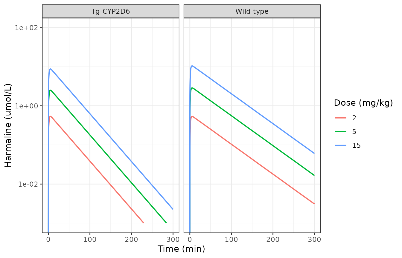
Replicates the shape of Figure 7A and 7B of Jiang 2016: simulated serum harmaline after 2, 5 and 15 mg/kg i.p.
Check 4: dose-proportionality and mass balance via PKNCA
Two quantitative claims in the Discussion (p. 501) are printed in the text, so they are non-circular gates rather than figure readings:
- harmaline exposure rises “almost 20-fold” going from 2 to 15 mg/kg;
- early-time (0-60 min) 5-MeO-DMT exposure at 10 mg/kg rises “only by 20%” when the harmaline dose rises from 2 to 15 mg/kg.
The first is a direct test of the dose-dependent bioavailability: the dose itself only rises 7.5-fold, so the rest must come from FH rising from 34.6% to 90.3%.
conc_har <- pk_sims |>
  filter(!is.na(Cc_harmaline)) |>
  transmute(id = paste(genotype, dose_harmaline), time, conc = Cc_harmaline,
            genotype, dose_harmaline)

dose_har <- conc_har |>
  group_by(id, genotype, dose_harmaline) |>
  summarise(time = 0, .groups = "drop")

o_conc <- PKNCA::PKNCAconc(conc_har, conc ~ time | id)
o_dose <- PKNCA::PKNCAdose(dose_har, ~ time | id)
res_har <- PKNCA::pk.nca(PKNCA::PKNCAdata(
  o_conc, o_dose,
  intervals = data.frame(start = 0, end = 300, auclast = TRUE, cmax = TRUE)
))

auc_har <- as.data.frame(res_har) |>
  filter(PPTESTCD == "auclast") |>
  left_join(distinct(conc_har, id, genotype, dose_harmaline), by = "id")

fold_wt <- with(
  auc_har[auc_har$genotype == "Wild-type", ],
  PPORRES[dose_harmaline == 15] / PPORRES[dose_harmaline == 2]
)

# Dose ratio 7.5 x bioavailability ratio (0.903 / 0.346 = 2.61) = 19.6.
stopifnot(fold_wt > 15, fold_wt < 24)
c(harmaline_auc_fold_2_to_15 = round(fold_wt, 1))
#> harmaline_auc_fold_2_to_15
#>                       19.6
The model gives a 19.6-fold rise, matching the paper’s “almost 20-fold”. A flat-bioavailability encoding would give only 7.5-fold, so this gate fails loudly if the FH lookup is wrong.
Mass balance closes the same loop from the other side: for a linear
disposition, CL x AUC(0-inf) must return the absorbed
dose.
mb <- pk_sims |>
  filter(genotype == "Wild-type") |>
  group_by(dose_harmaline) |>
  summarise(
    # Trapezoid over the simulated grid plus the analytic terminal tail.
    auc_last = sum(diff(time) * (head(Cc_harmaline, -1) + tail(Cc_harmaline, -1)) / 2),
    c_last = tail(Cc_harmaline, 1),
    .groups = "drop"
  ) |>
  mutate(
    lambda_z = 0.0962 / (2.43 + 2.86), # terminal slope of the 2-cmt system
    auc_inf = auc_last + c_last / lambda_z,
    absorbed = dose_harmaline / MW_HARMALINE * 1000 *
      c(0.346, 0.742, 0.903),
    recovered = 0.0962 * auc_inf,
    pct_err = 100 * (recovered - absorbed) / absorbed
  )

stopifnot(max(abs(mb$pct_err)) < 5)
mb |>
  select(dose_harmaline, absorbed, recovered, pct_err) |>
  rename("Dose (mg/kg)" = dose_harmaline, "F x Dose (umol/kg)" = absorbed,
         "CL x AUCinf (umol/kg)" = recovered, "Error (%)" = pct_err) |>
knitr::kable(digits = 2)| Dose (mg/kg) | F x Dose (umol/kg) | CL x AUCinf (umol/kg) | Error (%) |
|---|---|---|---|
| 2 | 3.23 | 3.23 | -0.02 |
| 5 | 17.32 | 17.31 | -0.02 |
| 15 | 63.22 | 63.20 | -0.02 |
Now the second printed claim, which exercises the competitive-inhibition terms.
ddi_sims <- bind_rows(lapply(c(2, 5, 15), function(dh) {
  simulate_arm(paste0("HAR ", dh, " + MEO 10"), dose_harmaline = dh,
               dose_meodmt = 10, tg = 0, tmax = 300, dt = 0.25)
}))

auc_meo_60 <- ddi_sims |>
  filter(time >= 15, time <= 60) |>
  group_by(dose_harmaline) |>
  summarise(
    auc = sum(diff(time) * (head(Cc_meodmt, -1) + tail(Cc_meodmt, -1)) / 2),
    .groups = "drop"
  )

meo_fold <- with(auc_meo_60, auc[dose_harmaline == 15] / auc[dose_harmaline == 2])

# Paper: "only increased by 20%"; anything near 1 rather than a large factor.
stopifnot(meo_fold > 1.0, meo_fold < 1.5)
c(meodmt_early_auc_fold_2_to_15 = round(meo_fold, 2))
#> meodmt_early_auc_fold_2_to_15
#>                          1.18
A 1.18-fold rise, against the paper’s ~1.2. The point the authors draw from this is that the late hyperpyrexia at toxic dose combinations cannot be attributed to 5-MeO-DMT exposure, because 5-MeO-DMT exposure barely moves while harmaline exposure moves 20-fold.
Check 5: replicating the thermoregulatory figures
Figure 2 – saline only
fig2 <- bind_rows(
  bind_rows(lapply(c(0, 1), function(tg) {
    simulate_arm("Baseline", tg = tg, tmax = 300)
  })),
  bind_rows(lapply(c(0, 1), function(tg) {
    simulate_arm("Saline", tg = tg, tmax = 300, inj_extra = TRUE,
                 t_second = 0)
  })),
  bind_rows(lapply(c(0, 1), function(tg) {
    # Two handling events: one at 0 and one at 15 min.
    ev <- rxode2::et(seq(0, 300, by = 0.5), cmt = "temp")
    ev <- rxode2::et(ev, amt = 1, cmt = "stress", time = 0)
    ev <- rxode2::et(ev, amt = 1, cmt = "stress", time = 15)
    d <- as.data.frame(ev)
    d$CYP2D6_TG <- tg
    d$INJ_REPEAT <- 1L
    d$CONMED_HARMALINE <- 0L
    d$DOSE_HARMALINE_MGKG <- 0
    out <- rxode2::rxSolve(mod, d, returnType = "data.frame")
    out$arm <- "Saline + saline"
    out$genotype <- ifelse(tg == 1, "Tg-CYP2D6", "Wild-type")
    out
  }))
)

fig2_peaks <- fig2 |>
  group_by(arm) |>
  summarise(peak = max(temp), t_peak = time[which.max(temp)], .groups = "drop")

stopifnot(
  # Single saline peaks near 37.1 degC around 15 min (Fig. 2, dashed line).
  abs(fig2_peaks$peak[fig2_peaks$arm == "Saline"] - 37.1) < 0.4,
  # A second injection must raise the peak above a single one.
  fig2_peaks$peak[fig2_peaks$arm == "Saline + saline"] >
    fig2_peaks$peak[fig2_peaks$arm == "Saline"],
  # The undosed baseline never shows a transient.
  fig2_peaks$peak[fig2_peaks$arm == "Baseline"] < 36.4
)
knitr::kable(fig2_peaks, digits = 2)| arm | peak | t_peak |
|---|---|---|
| Baseline | 36.25 | 300.0 |
| Saline | 37.06 | 13.0 |
| Saline + saline | 37.97 | 24.5 |
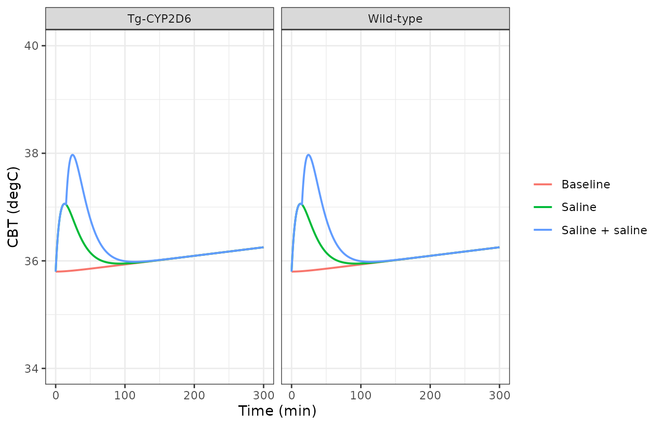
Replicates Figure 2 of Jiang 2016: CBT at baseline and after single or double saline injection.
Figure 3 – each drug alone
har_arms <- tidyr::crossing(dose = c(2, 5, 15), tg = c(0, 1))
fig3_har <- bind_rows(Map(
  function(dose, tg) {
    simulate_arm(paste0("HAR ", dose), dose_harmaline = dose, tg = tg,
                 tmax = 180)
  },
  har_arms$dose, har_arms$tg
))
meo_arms <- tidyr::crossing(dose = c(2, 10, 20), tg = c(0, 1))
fig3_meo <- bind_rows(Map(
  function(dose, tg) {
    simulate_arm(paste0("MEO ", dose), dose_meodmt = dose, tg = tg,
                 t_second = 0, tmax = 240)
  },
  meo_arms$dose, meo_arms$tg
))

meo_peaks <- fig3_meo |>
  group_by(genotype, dose_meodmt) |>
  summarise(peak = max(temp), .groups = "drop") |>
  mutate(fig3_peak = c(37.2, 37.55, 37.8, 37.2, 37.55, 37.8))

har_nadirs <- fig3_har |>
  group_by(genotype, dose_harmaline) |>
  summarise(nadir = min(temp), .groups = "drop")

stopifnot(
  # 5-MeO-DMT hyperthermia: digitised from Fig. 3C/D, so a loose bound.
  max(abs(meo_peaks$peak - meo_peaks$fig3_peak)) < 0.5,
  # Dose-ordered in both directions.
  all(diff(meo_peaks$peak[meo_peaks$genotype == "Wild-type"]) > 0),
  all(diff(har_nadirs$nadir[har_nadirs$genotype == "Wild-type"]) < 0),
  # The paper's central genotype finding: harmaline hypothermia is deeper in
  # wild-type mice, while 5-MeO-DMT hyperthermia is genotype-independent.
  har_nadirs$nadir[har_nadirs$genotype == "Wild-type" &
    har_nadirs$dose_harmaline == 15] <
    har_nadirs$nadir[har_nadirs$genotype == "Tg-CYP2D6" &
      har_nadirs$dose_harmaline == 15],
  max(abs(diff(meo_peaks$peak[meo_peaks$dose_meodmt == 20]))) < 0.1
)
knitr::kable(meo_peaks, digits = 2)| genotype | dose_meodmt | peak | fig3_peak |
|---|---|---|---|
| Tg-CYP2D6 | 2 | 37.13 | 37.20 |
| Tg-CYP2D6 | 10 | 37.44 | 37.55 |
| Tg-CYP2D6 | 20 | 37.73 | 37.80 |
| Wild-type | 2 | 37.13 | 37.20 |
| Wild-type | 10 | 37.45 | 37.55 |
| Wild-type | 20 | 37.73 | 37.80 |
knitr::kable(har_nadirs, digits = 2)| genotype | dose_harmaline | nadir |
|---|---|---|
| Tg-CYP2D6 | 2 | 35.80 |
| Tg-CYP2D6 | 5 | 35.48 |
| Tg-CYP2D6 | 15 | 33.67 |
| Wild-type | 2 | 35.80 |
| Wild-type | 5 | 35.13 |
| Wild-type | 15 | 32.63 |
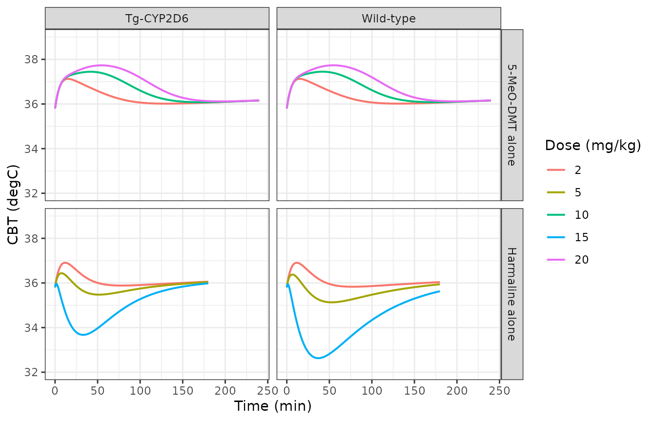
Replicates Figure 3 of Jiang 2016: harmaline-induced hypothermia (top) and 5-MeO-DMT-induced hyperthermia (bottom).
The wild-type nadir after 15 mg/kg harmaline is 32.63 degC against roughly 33.3 degC for the fitted line in Fig. 3A – see Errata.
Figure 4 – the biphasic combination response
Co-administering harmaline with 2 mg/kg 5-MeO-DMT is the paper’s signature result: hypothermia early (0-45 min), hyperthermia late (45-120 min).
fig4_arms <- tidyr::crossing(dose = c(2, 5, 15), tg = c(0, 1))
fig4 <- bind_rows(Map(
  function(dose, tg) {
    simulate_arm(paste0("HAR ", dose, " + MEO 2"), dose_harmaline = dose,
                 dose_meodmt = 2, tg = tg, tmax = 240)
  },
  fig4_arms$dose, fig4_arms$tg
))

biphasic <- fig4 |>
  group_by(genotype, dose_harmaline) |>
  summarise(
    early_peak = max(temp[time <= 20]),
    early_min = min(temp[time <= 45]),
    late_max = max(temp[time > 45 & time <= 120]),
    .groups = "drop"
  ) |>
  mutate(swing = late_max - early_min)

stopifnot(
  # The shape is genuinely biphasic: an early handling-driven rise, a fall, and
  # then a second, 5-MeO-DMT-driven peak.
  all(biphasic$early_peak > biphasic$early_min),
  all(biphasic$swing > 0.5),
  # More harmaline means a lower late peak: harmaline's hypothermic action
  # progressively offsets the 5-MeO-DMT hyperthermia. Strictly ordered in both
  # genotypes (WT 37.71 / 37.37 / 36.92; Tg 37.72 / 37.51 / 37.23).
  all(diff(biphasic$late_max[biphasic$genotype == "Wild-type"]) < 0),
  all(diff(biphasic$late_max[biphasic$genotype == "Tg-CYP2D6"]) < 0),
  # The same offset suppresses the early handling-driven peak
  # (WT 37.75 / 37.40 / 36.32; Tg 37.75 / 37.48 / 36.65).
  all(diff(biphasic$early_peak[biphasic$genotype == "Wild-type"]) < 0),
  all(diff(biphasic$early_peak[biphasic$genotype == "Tg-CYP2D6"]) < 0),
  # Genotype effect survives into the combination: at 15 mg/kg the wild-type
  # trough is the deeper one, because harmaline is cleared more slowly.
  biphasic$early_min[biphasic$genotype == "Wild-type" &
    biphasic$dose_harmaline == 15] <
    biphasic$early_min[biphasic$genotype == "Tg-CYP2D6" &
      biphasic$dose_harmaline == 15]
)
knitr::kable(biphasic, digits = 2)| genotype | dose_harmaline | early_peak | early_min | late_max | swing |
|---|---|---|---|---|---|
| Tg-CYP2D6 | 2 | 37.75 | 35.80 | 37.72 | 1.92 |
| Tg-CYP2D6 | 5 | 37.48 | 35.80 | 37.51 | 1.71 |
| Tg-CYP2D6 | 15 | 36.65 | 35.80 | 37.23 | 1.43 |
| Wild-type | 2 | 37.75 | 35.80 | 37.71 | 1.91 |
| Wild-type | 5 | 37.40 | 35.80 | 37.37 | 1.57 |
| Wild-type | 15 | 36.32 | 35.71 | 36.92 | 1.20 |
Two features are worth reading off that table. First, the early-phase
hypothermia is shallow here, and that is the model behaving as the paper
describes rather than a defect: the combination arms use the
repeat-handling regimen, which more than halves kS-H, and
they carry two handling events whose stress signal pushes temperature up
over the same window. Only the wild-type 15 mg/kg arm dips below its
starting temperature. Second, at low harmaline doses the early,
handling-driven peak is the taller of the two; what rising harmaline
does is push both peaks down monotonically, which is the hypothermic arm
progressively offsetting both the stress and the 5-MeO-DMT
hyperthermia.
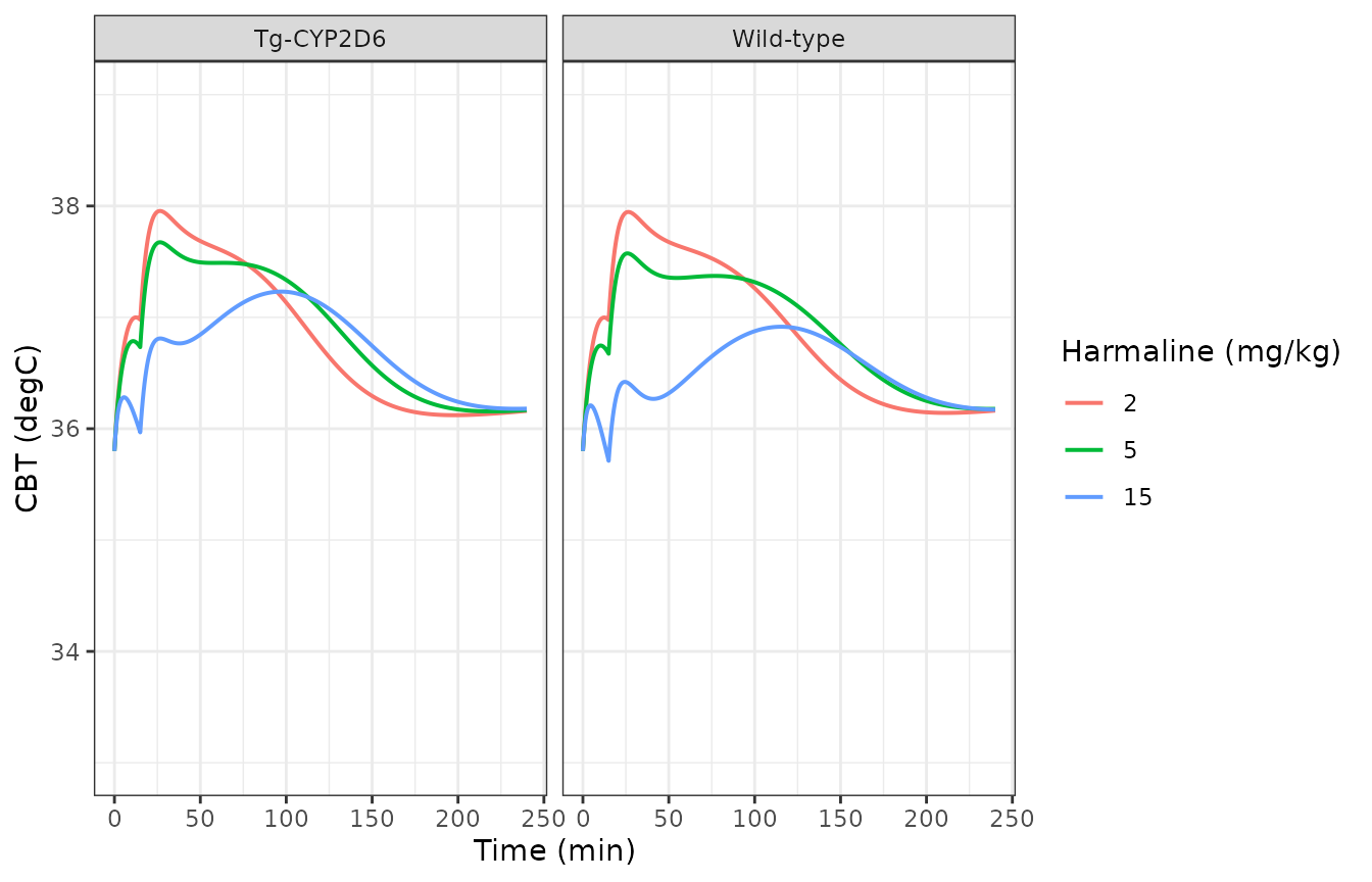
Replicates Figure 4E and 4F of Jiang 2016: harmaline plus 2 mg/kg 5-MeO-DMT.
Check 6: the 4-fold potency shift is wired to the right arm
SC50-M must take the DDI value only when harmaline is
actually present.
ec50_nonddi <- exp(mod$theta[["lec50_meodmt_nonddi"]])
ec50_ddi <- exp(mod$theta[["lec50_meodmt_ddi"]])

# Same 5-MeO-DMT dose, with and without harmaline pretreatment.
with_har <- simulate_arm("with", dose_harmaline = 5, dose_meodmt = 2, tmax = 240)
no_har <- simulate_arm("without", dose_meodmt = 2, t_second = 15, tmax = 240)

stopifnot(
  abs(ec50_nonddi - 1.88) < 1e-6,
  abs(ec50_ddi - 0.496) < 1e-6,
  abs(ec50_nonddi / ec50_ddi - 3.79) < 0.02,
  # The transduction signal driving thermogenesis must be larger under DDI.
  max(with_har$transit3) > max(no_har$transit3)
)
c(
  SC50_nonDDI = ec50_nonddi, SC50_DDI = ec50_ddi,
  fold = round(ec50_nonddi / ec50_ddi, 2)
)
#> SC50_nonDDI    SC50_DDI        fold
#>       1.880       0.496       3.790
Assumptions, deviations and errata
Clearance units.
CLother-H(0.0962) andCLCYP2D6-H(0.0608) are printed as “L/min” in Methods 2.4 while every neighbouring volume, clearance and Vmax carries “/kg”. They are encoded here as L/min/kg. Check 3 is the evidence: the per-kg reading reproduces the peak concentrations in the authors’ own Fig. 7A/B to within 5%, whereas an absolute-L/min reading would be roughly 30-fold low and could not produce the observed hypothermia at all. This is treated as a typographical omission in the source.Form of the two inhibition terms. The paper names
Ki(M)-HandKi(D)-Hbut never writes the inhibited rate equations. Fig. 1 draws both inhibition arrows terminating in a bar on the Km label of the respective pathway, which is competitive inhibition, so both are encoded asKm_app = Km * (1 + Cc_harmaline / Ki). The “other murine” route carries no inhibition arrow and is left uninhibited.Form of the CYP2D6 O-demethylation term. Likewise unwritten in the text. The Fig. 1 schematic prints it explicitly as
Vmax(D)-M x (1 + fmCYP2D6(D)), which is what the model implements.Residual error. Eq. (10) defines the variance model as
VAR = (sigma1 + sigma2 * Y)^2, a combined additive-plus-proportional SD, but no numeric sigma is printed in Table 1 or anywhere else in the paper. The structure is preserved and both SDs are held atfixed(0); a user re-fitting this model must supply their own starting values. (The printed Eq. (10) reads(sigma1 + sigma1 * Y)while the surrounding text defines bothsigma1andsigma2, so the second subscript is itself a typo in the source.)No inter-individual variability. The fit was naive-pooled, so the paper reports no IIV and none is invented. Every simulation here is deterministic.
Bioavailability away from the published doses.
FHis published only at 2, 5 and 15 mg/kg. The model reproduces those six values exactly and interpolates linearly between them, holding the nearest value outside the range. This is an encoding choice: the paper’s own external-validation arm (Fig. 5A/B) uses 10 mg/kg harmaline, a dose for which it reports noFH, and does not say what it used.Molecular weights. 214.26 g/mol (harmaline) and 218.30 g/mol (5-MeO-DMT) are chemical constants used only to convert the published mg/kg doses into the model’s umol/kg; they are not from the paper.
Deviation – depth of harmaline hypothermia at 15 mg/kg. The model reaches a wild-type nadir near 32.6 degC where the fitted line in Fig. 3A bottoms out around 33.3 degC (Tg-CYP2D6: 33.7 versus roughly 34.6 degC). Direction, timing and the genotype ordering are all reproduced, and the lower doses agree closely; the discrepancy is confined to the highest harmaline dose. Since the PK at that dose matches Fig. 7A to within 5%, the residual difference sits in the PD arm. It is recorded here rather than tuned away, and is excluded from the assertions above.
Not reproduced – the toxic dose combinations of Fig. 6. The authors state plainly that their model fails there, underestimating the early rise and overestimating the late fall in CBT for 5 or 15 mg/kg harmaline plus 10 mg/kg 5-MeO-DMT. That is a published limitation of the model, not of this encoding, and no attempt is made to match those profiles.
Upstream PK source. All PK parameters are fixed values carried over from the companion PK-interaction study (Jiang 2013, Drug Metab Dispos 41:975-86), and every one of them is reprinted in Methods 2.4 of this paper, which is where they were read from. The upstream paper itself is not open access; the structural forms it would have supplied are instead resolved from Fig. 1 as described above.
Known convention warning – the
tempobservation variable.checkModelConventions()emits one warning for this model: the single-output observation variabletempis not a registered canonical. That is deliberate. The standing convention is that a compartment canonical is promoted only once a second, independent paper uses the same state, so core body temperature is carried here inpaper_specific_compartmentsrather than minted as a library-wide canonical on the strength of one paper – particularly sincetempis a collision-prone token (a future model may want it for something else, and the paper’s own abbreviationCBTis an equally good candidate). The warning is the correct signal for a first sighting; the trigger to revisit is a second thermoregulation PK/PD model arriving in the library, at which point the state should be registered ininst/references/compartment-names.mdand this note removed. All other convention checks pass, and the four covariate columns this model introduces (CYP2D6_TG,INJ_REPEAT,CONMED_HARMALINE,DOSE_HARMALINE_MGKG) are registered ininst/references/covariate-columns.md.