Paclitaxel liposome PK and neutropenia (Zhou 2020)

Model and source

Zhou 2020 contributes two models, which are packaged separately because the authors fitted them in sequence: a population PK model for total plasma paclitaxel after paclitaxel liposome (Lipusu), and a logistic exposure-safety regression for neutropenia on the individual AUC derived from that PK model.

• Citation: Zhou H, Yan J, Chen W, Yang J, Liu M, Zhang Y, Shen X, Ma Y, Hu X, Wang Y, Du K, Li G. Population Pharmacokinetics and Exposure-Safety Relationship of Paclitaxel Liposome in Patients With Non-small Cell Lung Cancer. Front Oncol. 2020;10:1731 (issue dated 5 February 2021). doi:10.3389/fonc.2020.01731. Final estimates from Table 2; model structure confirmed against the NONMEM control stream in Supplementary Data Sheet 1.
• PK model: Three-compartment population PK model for total plasma paclitaxel (liposome-encapsulated plus released drug) after a 3-h intravenous infusion of paclitaxel liposome (Lipusu) 175 mg/m^2 in adults with squamous non-small cell lung cancer (Zhou 2020, n = 45). Linear first-order elimination from the central compartment, a deep and a shallow peripheral compartment, and between-subject variability on clearance only. No covariate was retained: age, sex, body weight, total bilirubin, albumin, serum creatinine, creatinine clearance and co-administration of aidi injection were all screened and rejected. The companion exposure-safety model is Zhou_2020_paclitaxel_liposomal_neutropenia.
• Exposure-safety model: Landmark logistic-regression exposure-safety model for neutropenia of CTCAE v4.0 grade 2 or worse (the source’s ‘grade > 1’) as a linear function of the individual total-paclitaxel AUC, in adults with squamous non-small cell lung cancer given paclitaxel liposome (Lipusu) 175 mg/m^2 as a 3-h infusion followed by platinum chemotherapy (Zhou 2020, n = 45). There is no PK layer and no ODE: the exposure metric is supplied as the AUC_PTX data column, which the source computed from each patient’s dose and post hoc clearance from the companion population PK model Zhou_2020_paclitaxel_liposomal. The exposure slope was significant at p = 0.0469.
• Article: https://doi.org/10.3389/fonc.2020.01731
• Supplement (NONMEM control stream, Data Sheet 1): https://www.frontiersin.org/articles/10.3389/fonc.2020.01731/full#supplementary-material

Population

Forty-five adults with squamous non-small cell lung cancer from a single centre in Beijing (Chinese Clinical Trial Registry ChiCTR2000029106) received paclitaxel liposome 175 mg/m^2 as a 3-h intravenous infusion on day 1 of a 3-week cycle, followed on day 2 by cisplatin 75 mg/m^2 or carboplatin AUC 4-5. The dose was rounded to the nearest vial size, giving 210, 240, 270 or 300 mg (4 / 29 / 31 / 24 administrations over the two sampled cycles). In cycle 2 the traditional Chinese medicine aidi injection was given before chemotherapy. Table 1 gives the baseline characteristics: median age 59 (36-75) years, median weight 71.5 (45-100) kg, 91% male, median creatinine clearance 101.1 (53.4-159.1) mL/min, total bilirubin 8.4 (2.3-35.5) umol/L and albumin 42.6 (30.7-50.5) g/L. Sparse samples were taken at 1.5, 3, 4, 6 and 21 h after the start of the infusion in each cycle, 349 concentrations in all; 43 patients completed cycle 2. The assay measured total paclitaxel (liposome-encapsulated plus released), LLOQ 10 ng/mL.

The same information is available programmatically via readModelDb("Zhou_2020_paclitaxel_liposomal")()$population.

Source trace

Equation / parameter	Value	Source location
Three-compartment structure, first-order elimination from central	n/a	Results ‘Model’; supplementary control stream (ADVAN6, $DES)
Pi = exp(PTV + eta_i) for every structural parameter	n/a	Methods ‘Model Development and Evaluation’; control stream $PK
CLi = exp(theta_CL + eta_CL) (only CL carries IIV)	n/a	Results ‘Model’ equation; control stream $OMEGA (all other diagonals 0 FIX)
lcl	log(21.55 L/h)	Table 2, CL
lvc	log(0.9248 L)	Table 2, Vc
lq (deep)	log(4.62 L/h)	Table 2, Q1; control stream CL2 / V2 pair
lvp (deep)	log(44.15 L)	Table 2, Vp1
lq2 (shallow)	log(15.85 L/h)	Table 2, Q2; control stream CL3 / V3 pair
lvp2 (shallow)	log(5.577 L)	Table 2, Vp2
etalcl	0.04264 (= 0.2065^2)	Table 2, IIV CL 20.65%
propSd	0.4455	Table 2, sigma1 44.55%; control stream Y = F*(1+EPS(1))
logit[P(NE > 1)] = a + b * AUC	n/a	Results ‘Exposure-Safety Analysis’ equation
logit_ref (a)	-3.5008	Table 3
e_auc_logit (b)	0.372 per mg*h/L	Table 3; units from Figure 5 x-axis
AUC_PTX = Dose / CL_i	n/a	Methods ‘Exposure-Safety Analysis’ (‘individual post hoc PK parameters and dosage’)

Virtual cohort

Original observed data are not publicly available. The cohort below draws the administered dose from the Table 1 dose frequencies. No covariate enters either model, so no other characteristic needs to be simulated.

set.seed(20210205)
n_sub <- 200L
dose_levels <- c(210, 240, 270, 300)
dose_weights <- c(4, 29, 31, 24) # Table 1, administrations per dose

obs_times <- sort(unique(c(
  seq(0, 3, by = 0.05),
  seq(3.01, 3.5, by = 0.01),
  seq(3.55, 6, by = 0.05),
  seq(6.25, 24, by = 0.25),
  seq(25, 72, by = 1)
)))

subjects <- tibble::tibble(
  id = seq_len(n_sub),
  dose = sample(dose_levels, n_sub, replace = TRUE, prob = dose_weights)
) |>
  mutate(treatment = paste0(dose, " mg"))

dose_rows <- subjects |>
  mutate(time = 0, amt = dose, rate = dose / 3, evid = 1L, cmt = "central")
obs_rows <- subjects |>
  tidyr::crossing(time = obs_times) |>
  mutate(amt = 0, rate = 0, evid = 0L, cmt = "central")
events <- bind_rows(dose_rows, obs_rows) |>
  arrange(id, time, desc(evid)) |>
  as.data.frame()

stopifnot(!anyDuplicated(unique(events[, c("id", "time", "evid")])))
table(subjects$treatment)
#> 
#> 210 mg 240 mg 270 mg 300 mg 
#>      9     71     78     42

Simulation

mod <- readModelDb("Zhou_2020_paclitaxel_liposomal")

# The model must be integrated as written (three d/dt() states), not
# silently converted to a closed-form solution.
stopifnot(is.null(rxode2::rxode(mod)$linCmt))
#> ℹ parameter labels from comments will be replaced by 'label()'

sim <- rxode2::rxSolve(
  mod,
  events = events,
  keep = "treatment",
  rtol = 1e-10,
  atol = 1e-12
) |>
  as.data.frame()
#> ℹ parameter labels from comments will be replaced by 'label()'

Typical-value profile

ev_typ <- data.frame(
  id = 1L,
  time = c(0, obs_times),
  amt = c(240, rep(0, length(obs_times))),
  rate = c(80, rep(0, length(obs_times))),
  evid = c(1L, rep(0L, length(obs_times))),
  cmt = "central"
)
sim_typ <- rxode2::rxSolve(
  rxode2::zeroRe(mod),
  events = ev_typ,
  rtol = 1e-10,
  atol = 1e-12
) |>
  as.data.frame()
#> ℹ parameter labels from comments will be replaced by 'label()'
#> ℹ omega/sigma items treated as zero: 'etalcl'

typ_at <- function(t) {
  v <- sim_typ$Cc[abs(sim_typ$time - t) < 1e-9]
  if (length(v) != 1L) {
    stop("no unique typical-value row at time ", t)
  }
  v
}

# Observed medians read from the solid line of Figure 3 (mixed 210-300 mg
# doses; Figure 3 plots every sample at its actual time).
fig3 <- tibble::tribble(
  ~time, ~observed_median,
  1.5, 3.3,
  6, 0.13,
  21, 0.032
) |>
  mutate(
    typical_240mg = vapply(time, typ_at, numeric(1)),
    ratio = typical_240mg / observed_median
  )
knitr::kable(
  fig3 |>
    rename(
      "Time (h)" = time,
      "Figure 3 observed median (mg/L)" = observed_median,
      "Model typical value, 240 mg (mg/L)" = typical_240mg,
      "Ratio" = ratio
    ),
  digits = 3,
  caption = "Typical-value concentrations against the Figure 3 observed median."
)

Typical-value concentrations against the Figure 3 observed median.

Time (h)	Figure 3 observed median (mg/L)	Model typical value, 240 mg (mg/L)	Ratio
1.5	3.300	3.020	0.915
6.0	0.130	0.127	0.975
21.0	0.032	0.033	1.037

# A mis-transcribed CL, volume or unit shifts at least one of these three
# phases by far more than the precision of a figure read.
stopifnot(all(fig3$ratio > 0.7 & fig3$ratio < 1.4))

Replicate published figures

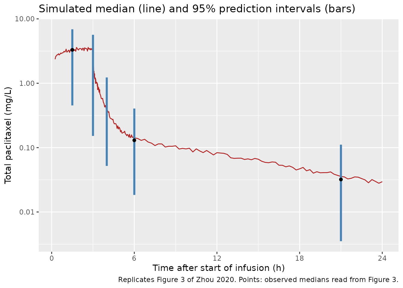
# Replicates Figure 3 of Zhou 2020: VPC of total paclitaxel concentrations.
# `sim` carries residual error, as the VPC prediction intervals do. The
# median is drawn on the full grid; the 2.5th-97.5th percentile intervals are
# drawn at the five nominal sampling times, pooling simulated observations
# within +/- 0.25 h of each (600 to 6200 values per time) as the binned
# Figure 3 does.
vpc_median <- sim |>
  filter(time >= 0.25, time <= 24) |>
  group_by(time) |>
  summarise(Q50 = median(sim), .groups = "drop")

nominal <- c(1.5, 3, 4, 6, 21)
vpc_pi <- sim |>
  tidyr::crossing(nominal = nominal) |>
  filter(abs(time - nominal) <= 0.25) |>
  group_by(nominal) |>
  summarise(
    n = n(),
    Q025 = quantile(sim, 0.025),
    Q50 = median(sim),
    Q975 = quantile(sim, 0.975),
    .groups = "drop"
  )
stopifnot(nrow(vpc_pi) == 5L, all(vpc_pi$n >= 600))

# A proportional error with SD 0.4455 draws a negative observation about 1.3%
# of the time (P(eps < -1)), so a 2.5th percentile can occasionally fall at or
# below zero. Floor it for the log axis only; the table shows the raw value.
vpc_plot <- vpc_pi |> mutate(Q025 = pmax(Q025, 1e-3))

ggplot(vpc_median, aes(time, Q50)) +
  geom_line(colour = "firebrick") +
  geom_linerange(
    data = vpc_plot,
    aes(x = nominal, ymin = Q025, ymax = Q975),
    inherit.aes = FALSE,
    colour = "steelblue",
    linewidth = 1.2
  ) +
  geom_point(data = fig3, aes(time, observed_median), inherit.aes = FALSE) +
  scale_y_log10() +
  scale_x_continuous(breaks = seq(0, 24, by = 6)) +
  labs(
    x = "Time after start of infusion (h)",
    y = "Total paclitaxel (mg/L)",
    title = "Simulated median (line) and 95% prediction intervals (bars)",
    caption = paste(
      "Replicates Figure 3 of Zhou 2020. Points: observed medians read",
      "from Figure 3."
    )
  )

knitr::kable(
  vpc_pi |>
    select(-n) |>
    rename(
      "Nominal time (h)" = nominal,
      "2.5th percentile (mg/L)" = Q025,
      "Median (mg/L)" = Q50,
      "97.5th percentile (mg/L)" = Q975
    ),
  digits = 3,
  caption = "Simulated observation percentiles at the nominal sampling times."
)

Simulated observation percentiles at the nominal sampling times.

Nominal time (h)	2.5th percentile (mg/L)	Median (mg/L)	97.5th percentile (mg/L)
1.5	0.452	3.236	6.896
3.0	0.152	1.497	5.659
4.0	0.052	0.390	1.231
6.0	0.018	0.145	0.405
21.0	0.004	0.035	0.111

The concentration falls roughly ten-fold within the first hour after the end of the infusion: with Vc = 0.92 L the initial disposition half-life is about one minute. This is why the paper’s 3-h (‘immediately at the end of infusion’) samples in Figure 3 span more than an order of magnitude, and why a few minutes of sampling delay matters when comparing against those samples.

PKNCA validation

sim_nca <- sim |>
  filter(!is.na(Cc)) |>
  select(id, time, Cc, treatment)
sim_nca <- bind_rows(
  sim_nca,
  sim_nca |> distinct(id, treatment) |> mutate(time = 0, Cc = 0)
) |>
  distinct(id, treatment, time, .keep_all = TRUE) |>
  arrange(id, treatment, time)

# Integrator undershoot in the far tail is noise; floor it before NCA.
stopifnot(all(sim_nca$Cc >= -1e-6 * max(sim_nca$Cc)))
sim_nca <- sim_nca |>
  mutate(Cc = pmax(Cc, 0)) |>
  group_by(id) |>
  filter(time <= time[which.max(Cc)] | Cc >= 1e-6 * max(Cc)) |>
  ungroup()

conc_obj <- PKNCA::PKNCAconc(sim_nca, Cc ~ time | treatment + id)
dose_obj <- PKNCA::PKNCAdose(
  events |> filter(evid == 1) |> select(id, time, amt, treatment),
  amt ~ time | treatment + id
)
intervals <- data.frame(
  start = 0,
  end = Inf,
  cmax = TRUE,
  tmax = TRUE,
  aucinf.obs = TRUE,
  half.life = TRUE
)
nca_res <- PKNCA::pk.nca(PKNCA::PKNCAdata(conc_obj, dose_obj, intervals = intervals))

nca_wide <- as.data.frame(nca_res) |>
  filter(PPTESTCD %in% c("cmax", "tmax", "aucinf.obs", "half.life")) |>
  select(id, treatment, PPTESTCD, PPORRES) |>
  tidyr::pivot_wider(names_from = PPTESTCD, values_from = PPORRES)

nca_wide |>
  group_by(treatment) |>
  summarise(
    n = n(),
    cmax = median(cmax),
    tmax = median(tmax),
    aucinf.obs = median(aucinf.obs),
    half.life = median(half.life),
    .groups = "drop"
  ) |>
  rename(
    "Dose" = treatment,
    "N" = n,
    "Cmax (mg/L)" = cmax,
    "Tmax (h)" = tmax,
    "AUC0-inf (mg*h/L)" = aucinf.obs,
    "Terminal t1/2 (h)" = half.life
  ) |>
  knitr::kable(digits = 2, caption = "Simulated NCA medians by dose.")

Simulated NCA medians by dose.

Dose	N	Cmax (mg/L)	Tmax (h)	AUC0-inf (mg*h/L)	Terminal t1/2 (h)
210 mg	9	2.89	3	10.20	8.13
240 mg	71	3.38	3	11.98	8.17
270 mg	78	3.71	3	13.08	8.13
300 mg	42	3.91	3	13.66	8.03

Zhou 2020 reports no NCA table, so there is no published NCA to compare against. Two checks stand in for it. First, for a linear model each subject’s AUC0-inf must equal Dose / CL_i, which ties the NCA to the individual clearance and to the dose units:

# One row per subject: the individual clearance from the solve and the dose
# from the per-subject cohort table (a one-to-one join on id).
cl_by_id <- sim |>
  group_by(id) |>
  summarise(cl = first(cl), .groups = "drop") |>
  inner_join(subjects |> select(id, dose), by = "id")
stopifnot(nrow(cl_by_id) == n_sub)

auc_check <- nca_wide |>
  select(id, aucinf.obs) |>
  inner_join(cl_by_id, by = "id") |>
  mutate(ratio = aucinf.obs * cl / dose)
stopifnot(nrow(auc_check) == n_sub)
summary(auc_check$ratio)
#>    Min. 1st Qu.  Median    Mean 3rd Qu.    Max. 
#>  0.9977  0.9984  0.9986  0.9986  0.9988  0.9992

# Trapezoidal error on the one-minute distribution phase is well under 1%
# on this grid; a wrong dose or clearance unit moves the ratio by 1000-fold.
stopifnot(
  abs(median(auc_check$ratio) - 1) < 0.01,
  quantile(abs(auc_check$ratio - 1), 0.9) < 0.02
)

Second, the Discussion converts the population clearance to a body-surface basis, 21.55 L/h / 1.84 m^2 = 11.71 L/h/m^2, and compares it with 12.3 +/- 2.7 L/h/m^2 from an earlier Lipusu report:

cl_typ <- exp(rxode2::rxode(mod)$theta[["lcl"]])
#> ℹ parameter labels from comments will be replaced by 'label()'
cl_bsa <- cl_typ / 1.84
cl_bsa
#> [1] 11.71196
stopifnot(abs(cl_bsa - 11.71) < 0.01)

Exposure-safety model

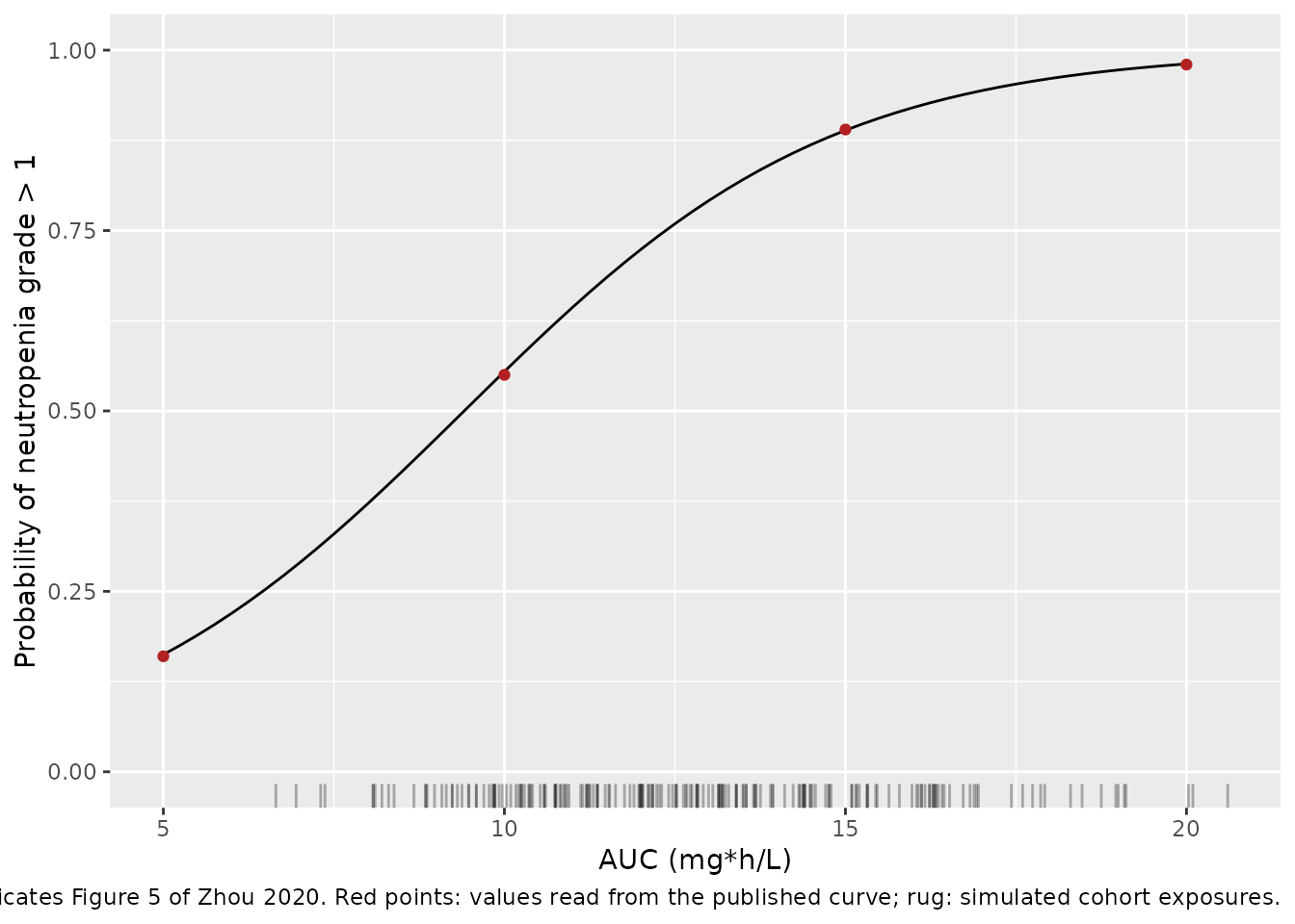
The Figure 5 exposures (x-axis, mg*h/L) are the individual AUCs. They are recomputed here as Dose / CL_i for the simulated cohort and passed to the neutropenia model as the AUC_PTX column.

er_mod <- readModelDb("Zhou_2020_paclitaxel_liposomal_neutropenia")

# The logistic model has no random effects by design, so rxode2's
# "multi-subject simulation without omega" warning is expected; muffle that
# one message and let any other warning through.
solve_er <- function(data) {
  withCallingHandlers(
    rxode2::rxSolve(er_mod, events = data, keep = "AUC_PTX"),
    warning = function(w) {
      if (grepl("without 'omega'", conditionMessage(w), fixed = TRUE)) {
        invokeRestart("muffleWarning")
      }
    }
  ) |>
    as.data.frame()
}

er_data <- cl_by_id |>
  mutate(time = 0, AUC_PTX = dose / cl) |>
  select(id, time, AUC_PTX)

quantile(er_data$AUC_PTX, c(0.05, 0.5, 0.95))
#>        5%       50%       95% 
#>  8.659573 12.666580 17.940683

# Figure 5 plots observed exposures from about 7.7 to 17 mg*h/L, centred
# near 12. The median of the simulated distribution is robust to the draw.
stopifnot(
  median(er_data$AUC_PTX) > 10,
  median(er_data$AUC_PTX) < 14
)

er_sim <- solve_er(er_data)
mean(er_sim$prob_neutropenia_grade2)
#> [1] 0.7385482

# Replicates Figure 5 of Zhou 2020: probability of neutropenia grade > 1
# against AUC.
curve_data <- data.frame(id = 1L, time = 0, AUC_PTX = seq(5, 20, by = 0.25))
curve_data$id <- seq_len(nrow(curve_data))
curve <- solve_er(curve_data)

curve_at <- function(a) {
  v <- curve$prob_neutropenia_grade2[abs(curve$AUC_PTX - a) < 1e-9]
  if (length(v) != 1L) {
    stop("no unique curve row at AUC ", a)
  }
  v
}

# Probabilities read from the fitted curve of Figure 5.
fig5 <- tibble::tribble(
  ~AUC_PTX, ~figure5,
  5, 0.16,
  10, 0.55,
  15, 0.89,
  20, 0.98
) |>
  mutate(
    model = vapply(AUC_PTX, curve_at, numeric(1))
  )

ggplot(curve, aes(AUC_PTX, prob_neutropenia_grade2)) +
  geom_line() +
  geom_point(data = fig5, aes(AUC_PTX, figure5), colour = "firebrick") +
  geom_rug(data = er_sim, aes(AUC_PTX), inherit.aes = FALSE, alpha = 0.3) +
  coord_cartesian(ylim = c(0, 1)) +
  labs(
    x = "AUC (mg*h/L)",
    y = "Probability of neutropenia grade > 1",
    caption = paste(
      "Replicates Figure 5 of Zhou 2020. Red points: values read from the",
      "published curve; rug: simulated cohort exposures."
    )
  )

knitr::kable(
  fig5 |>
    rename(
      "AUC (mg*h/L)" = AUC_PTX,
      "Figure 5 curve" = figure5,
      "Model" = model
    ),
  digits = 3
)

AUC (mg*h/L)	Figure 5 curve	Model
5	0.16	0.162
10	0.55	0.555
15	0.89	0.889
20	0.98	0.981

# Deterministic: the logistic curve has no random component. A sign or
# decimal error in either Table 3 coefficient moves these by >0.1.
stopifnot(all(abs(fig5$model - fig5$figure5) < 0.03))

Assumptions and deviations

• Year. The article is in volume 10 (2020) of Frontiers in Oncology, which is the year PubMed and Europe PMC index it under (PMID 33614470) and the year in its DOI, so the models are named Zhou_2020_*. The issue itself is dated 5 February 2021, and the article’s own suggested citation gives 2021.
• IIV scale. Table 2 prints the CL variability as 20.65%. It is encoded as the standard deviation of eta, omega^2 = 0.2065^2 = 0.04264. The supplementary control stream’s $OMEGA value for CL (0.0427, whose square root is 20.66%) supports this reading over log(CV^2 + 1), which would give 0.0418.
• Control stream values are initial estimates. The $THETA block of the supplementary stream (for example exp(3.09) = 21.98 L/h for CL) differs from Table 2 in the third digit, so it holds starting values. The stream was used only to confirm the model structure and the deep/shallow compartment mapping; all numbers come from Table 2.
• Compartment naming. The paper’s deep compartment (Vp1, Q1) is peripheral1 (vp, q) and its shallow compartment (Vp2, Q2) is peripheral2 (vp2, q2), following the paper’s numbering.
• Cycles. The PK model pools both cycles with no between-occasion variability and no cycle or aidi effect, so one cycle is simulated. The 21-day interval is more than 60 terminal half-lives, so there is no accumulation between cycles.
• AUC for the exposure-safety model. The source says only that the AUC was computed from the individual post hoc PK parameters and the dose. For a linear model the single-dose AUC0-inf is Dose / CL_i; which cycle’s dose and clearance were used, and whether per-cycle AUCs were combined, is not stated. Figure 5 plots one exposure per patient in the 7.7-17 mg*h/L range, which matches a single-cycle AUC.
• Neutropenia endpoint. ‘Grade > 1’ is encoded as grade 2 or worse (prob_neutropenia_grade2). The source took the event from electronic medical records by CTCAE v4.0, with any cycle of platinum doublet therapy contributing; the platinum exposure is not in the model.
• Placeholder residual. The logistic model was fitted with a Bernoulli likelihood and has no residual error. addSd_prob_neutropenia_grade2 = 0.001 (fixed) exists only so the nlmixr2 observation machinery accepts the model; it is not a published quantity.
• Figure reads. The Figure 3 observed medians and the Figure 5 curve values used in the checks above were read from the published figures by the maintainers and are approximate; the checks’ tolerances allow for this.
• Errata. No correction notice for this article was found as of 2026-09-27.