Model and source
- Citation: Fuhr LM, Marok FZ, Mees M, Mahfoud F, Selzer D, Lehr T. (2022). A Physiologically Based Pharmacokinetic and Pharmacodynamic Model of the CYP3A4 Substrate Felodipine for Drug-Drug Interaction Modeling. Pharmaceutics 14(7):1474. doi:10.3390/pharmaceutics14071474. Circadian baseline structure and amplitudes from Chae D, Kim Y, Park K (diastolic blood pressure) and Lott D et al. (heart rate), as cited by Fuhr 2022 (references 28 and 29).
- Description: Direct-effect pharmacodynamic model of felodipine on diastolic blood pressure (DBP) and heart rate (HR) in healthy and hypertensive adults, the PD layer of the Fuhr 2022 parent-metabolite PBPK/PD model. Each endpoint rides a cosinor circadian baseline (DBP: 24 h + 12 h harmonics after Chae et al.; HR: one 24 h harmonic after Lott et al.), scaled multiplicatively by the 24 h mean, from which felodipine subtracts a hyperbolic Emax effect (DBP) or to which it adds a sigmoid Emax effect (HR), both driven directly by the felodipine plasma concentration with no effect delay. Only this PD layer is reproduced here: the PBPK layer is a PK-Sim / MoBi whole-body model whose organ volumes, blood flows, partition coefficients and CYP3A4 expression profile are platform database outputs the paper does not print, so the felodipine plasma concentration is supplied by the user as the canonical driver covariate CEFFECT (umol/L) rather than generated by a PK model in this file. The 24 h means, circadian phases and amplitudes are the cross-study summary values of Table 3; the paper re-optimised the means and phases for every simulated study (supplementary Table S5). No inter-individual variability and no residual-error model are reported, so both are zero.
- Article: https://doi.org/10.3390/pharmaceutics14071474 (open access, PMC9322514)
- Supplement: https://www.mdpi.com/article/10.3390/pharmaceutics14071474/s1 (reference manual; Section 1.6 gives the PD equations S16-S22, Tables S5 and S6 the PD parameters)
Felodipine is a dihydropyridine calcium-channel blocker whose blood-pressure effect tracks its plasma concentration directly. Fuhr 2022 built a parent-metabolite PBPK model of felodipine and dehydrofelodipine in PK-Sim / MoBi (Open Systems Pharmacology Suite 9.1) and extended it with a PD model of diastolic blood pressure (DBP) and heart rate (HR). The PBPK model was then used to predict CYP3A4 drug-drug interactions with erythromycin, itraconazole, carbamazepine and phenytoin.
Only the PD layer is packaged here. The PBPK layer
is a platform whole-body model: its organ volumes, blood flows, tissue
partition coefficients (Rodgers-Rowland / Schmitt methods) and CYP3A4
expression profile are PK-Sim database outputs that the paper does not
tabulate, so it cannot be rebuilt from the publication. The PD layer, by
contrast, is printed in full (supplementary Equations S16-S22, main-text
Table 3). Its only input from the PBPK layer is the felodipine plasma
concentration. Here that concentration is supplied by the user as the
time-varying covariate CEFFECT (umol/L).
Population
The PD layer was built from 30 DBP-time and 22 HR-time profiles taken from 17 published clinical studies (Results 3.2; Table 1). Of these, 18 DBP and 18 HR profiles came from healthy volunteers and 12 DBP and 4 HR profiles from patients with essential hypertension, many of whom were also taking other antihypertensives (supplementary Table S1, footnote c). Felodipine was given as 1-3 mg intravenous infusions or as 0.83-40 mg oral solution, immediate-release tablet or extended-release tablet, in single or multiple doses. All data are means digitised from the literature. No individual data were used, so the total number of individuals is not reported. The healthy-volunteer cohorts in Table S1 are mostly young men (per-study mean ages 24-33 years); the hypertensive cohorts are older.
The same information is available programmatically via
readModelDb("Fuhr_2022_felodipine")()$population.
Source trace
| Equation / parameter | Value | Source location |
|---|---|---|
circ_dbp (24 h + 12 h cosinor) |
n/a | Supplement Eq. S16 (structure from Chae et al., ref. 28) |
dbp = e0_dbp * (1 + circ_dbp) - eff_dbp |
n/a | Supplement Eq. S17 and S21 |
circ_hr (24 h cosinor) |
n/a | Supplement Eq. S18 (structure from Lott et al., ref. 29) |
hr = e0_hr * (1 + circ_hr) + eff_hr |
n/a | Supplement Eq. S19 and S22 |
eff = emax * C^h / (ec50^h + C^h) |
n/a | Main-text Eq. 1 = supplement Eq. S20 |
lemax_dbp |
log(56.18 mmHg) | Table 3 (and Table S6), DBP Emax |
lec50_dbp |
log(0.04 umol/L) | Table 3, DBP EC50; “40 nmol/L” in the Discussion |
| DBP Hill coefficient | 1 (not a parameter) | Table 3 lists h for the HR model only |
amp24_dbp |
0.0214 (fixed) | Table 3, amp24 = 2.14 % (literature, ref. 28) |
amp12_dbp |
0.0593 (fixed) | Table 3, amp12 = 5.93 % (literature, ref. 28) |
phase24_dbp |
5.28 h | Table 3, mean (SD 2.10) of per-study values |
phase12_dbp |
0.16 h | Table 3, mean (SD 2.10) of per-study values |
le0_dbp |
log(70.4 mmHg) | Table 3, BPmean, healthy individuals |
e_hypert_e0_dbp |
log(91.9 / 70.4) | Table 3, BPmean for hypertensive individuals (footnote b) |
lemax_hr |
log(39.71 bpm) | Table 3, HR Emax |
lec50_hr |
log(0.05 umol/L) | Table 3, HR EC50 |
lhill_hr |
log(1.40) | Table 3, HR Hill coefficient |
amp_hr |
0.063 (fixed) | Table 3, amp = 6.3 % (literature, ref. 29) |
phase_hr |
11.8 h | Table 3, mean (SD 5.13) of per-study values |
le0_hr |
log(62.2 bpm) | Table 3, HRmean, healthy individuals |
e_hypert_e0_hr |
log(66.4 / 62.2) | Table 3, HRmean for hypertensive individuals (footnote b) |
addSd_dbp, addSd_hr
|
0 (fixed) | No residual-error model reported |
| Per-study BPmean, HRmean and phases | Table S5 | Used below to replicate Figure 4 |
| Felodipine molecular weight | 384.25 g/mol | Table 2 (converts ng/mL to umol/L) |
Deterministic structure checks
The model has no random effects, so every check below is exact.
mod <- readModelDb("Fuhr_2022_felodipine")
mw <- 384.25 # g/mol, Fuhr 2022 Table 2

grid <- expand.grid(
  time = seq(0, 24, by = 0.25),
  CEFFECT = c(0, 0.04, 0.05),
  DIS_HYPERT = c(0, 1)
)
ev_grid <- grid |>
  mutate(id = as.integer(interaction(CEFFECT, DIS_HYPERT, drop = TRUE)), evid = 0, amt = 0) |>
  arrange(id, time)
sim_grid <- as.data.frame(rxSolve(mod, ev_grid, keep = c("DIS_HYPERT")))
#> Warning: multi-subject simulation without without 'omega'

# Placebo 24 h means equal the Table 3 BPmean / HRmean values: the cosine
# harmonics average to zero over a whole 24 h period.
placebo_means <- sim_grid |>
  filter(CEFFECT == 0, time < 24) |>
  group_by(DIS_HYPERT) |>
  summarise(dbp_mean = mean(dbp), hr_mean = mean(hr), .groups = "drop")
knitr::kable(placebo_means, digits = 3)| DIS_HYPERT | dbp_mean | hr_mean |
|---|---|---|
| 0 | 70.4 | 62.2 |
| 1 | 91.9 | 66.4 |
stopifnot(
  abs(placebo_means$dbp_mean[placebo_means$DIS_HYPERT == 0] - 70.4) < 1e-6,
  abs(placebo_means$dbp_mean[placebo_means$DIS_HYPERT == 1] - 91.9) < 1e-6,
  abs(placebo_means$hr_mean[placebo_means$DIS_HYPERT == 0] - 62.2) < 1e-6,
  abs(placebo_means$hr_mean[placebo_means$DIS_HYPERT == 1] - 66.4) < 1e-6
)

# At CEFFECT = EC50 the drug effect is exactly Emax / 2 at every time point.
eff <- sim_grid |>
  filter(CEFFECT > 0) |>
  select(time, CEFFECT, DIS_HYPERT, eff_dbp, eff_hr)
stopifnot(
  all(abs(eff$eff_dbp[eff$CEFFECT == 0.04] - 56.18 / 2) < 1e-8),
  all(abs(eff$eff_hr[eff$CEFFECT == 0.05] - 39.71 / 2) < 1e-8)
)
Exposure-response with the Table 3 typical values
conc_nM <- c(0, 10^seq(-1, 3, length.out = 120))
ev_er <- data.frame(
  id = seq_along(conc_nM), time = 0, evid = 0, amt = 0,
  CEFFECT = conc_nM / 1000, DIS_HYPERT = 0
)
sim_er <- as.data.frame(rxSolve(mod, ev_er))
#> Warning: multi-subject simulation without without 'omega'
sim_er |>
  mutate(conc_nM = CEFFECT * 1000) |>
  filter(conc_nM > 0) |>
  select(conc_nM, `DBP decrease (mmHg)` = eff_dbp, `HR increase (beats/min)` = eff_hr) |>
  pivot_longer(-conc_nM) |>
  ggplot(aes(conc_nM, value)) +
  geom_line() +
  geom_vline(
    data = data.frame(
      name = c("DBP decrease (mmHg)", "HR increase (beats/min)"),
      ec50 = c(40, 50)
    ),
    aes(xintercept = ec50), linetype = "dashed"
  ) +
  facet_wrap(~name, scales = "free_y") +
  scale_x_log10() +
  labs(
    x = "Felodipine plasma concentration (nmol/L)", y = "Drug effect",
    caption = "Dashed lines: EC50 (Fuhr 2022 Table 3)."
  ) +
  theme_bw()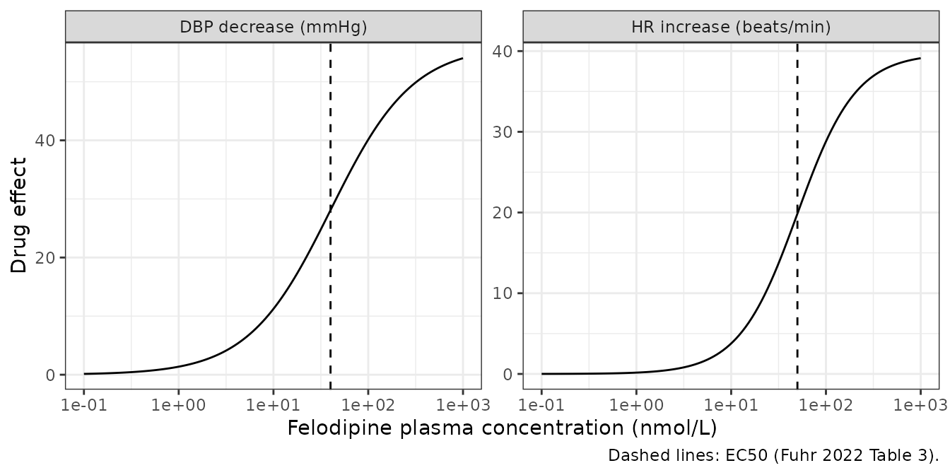
At 20 nmol/L (about 7.7 ng/mL), a typical peak after a 10-20 mg extended-release tablet, the model predicts a DBP decrease of 18.7 mmHg and an HR increase of 8.6 beats/min.
Replicating Figure 4
Figure 4 of Fuhr 2022 shows, for three studies, the PBPK-predicted felodipine plasma concentration (panels a-c) together with the predicted DBP (d-f) and HR (g-i) curves. Panels a, d-i are vector graphics in the article PDF. The maintainers extracted the model-prediction lines from the vector paths, with each axis calibrated on its tick marks, and resampled them onto a common time grid. Panels b and c are embedded raster images and were not digitised. The curves below are therefore the paper’s own predictions, not observed data.
Fuhr 2022 re-optimised the 24 h means and phases for every simulated study. Each replication therefore overrides the Table 3 means with that study’s Table S5 values:
- Edgar 1987 (healthy, oral solution 5 / 15 / 40 mg): BPmean 69.57 mmHg, phase12 0.95 h, phase24 6.07 h; HRmean 56.81 bpm, phaseHR 18.48 h.
- Blychert 1990 (hypertensive, 20 mg extended-release tablet once daily, day 15): BPmean 95.88 mmHg, phase12 1.01 h, phase24 6.13 h; HRmean 60.92 bpm, phaseHR 15.24 h.
- Hedner 1986 (hypertensive, 5 then 10 mg tablet twice daily, day 28): BPmean 87.70 mmHg, phase12 -0.02 h, phase24 5.10 h; HRmean 66.13 bpm, phaseHR 13.63 h.
Because these per-study means replace le0_dbp and
le0_hr directly, DIS_HYPERT is kept at 0 in
every replication. Setting it to 1 would apply the Table 3
hypertensive/healthy ratio a second time.
edgar <- data.frame(
  time = c(0.0, 0.1, 0.2, 0.3, 0.4, 0.5, 0.6, 0.7, 0.8, 0.9, 1.0, 1.1, 1.2, 1.3, 1.4, 1.5, 1.6, 1.7, 1.8, 1.9, 2.0, 2.1, 2.2, 2.3, 2.4, 2.5, 2.6, 2.7, 2.8, 2.9, 3.0, 3.5, 4.0, 4.5, 5.0, 5.5, 6.0, 6.5, 7.0, 7.5, 8.0, 8.5, 9.0, 9.5, 10.0, 10.5, 11.0),
  conc_5 = c(0.00, 1.16, 3.83, 5.25, 5.55, 5.27, 4.77, 4.23, 3.73, 3.31, 2.96, 2.68, 2.45, 2.27, 2.11, 1.99, 1.88, 1.78, 1.70, 1.62, 1.55, 1.49, 1.42, 1.37, 1.32, 1.27, 1.22, 1.17, 1.13, 1.09, 1.05, 0.88, 0.75, 0.65, 0.56, 0.49, 0.43, 0.39, 0.35, 0.31, 0.29, 0.26, 0.24, 0.22, 0.21, 0.19, 0.18),
  conc_15 = c(0.00, 2.96, 10.77, 16.28, 17.51, 16.71, 15.14, 13.42, 11.82, 10.46, 9.33, 8.43, 7.70, 7.12, 6.63, 6.23, 5.88, 5.58, 5.32, 5.08, 4.86, 4.65, 4.47, 4.29, 4.12, 3.96, 3.82, 3.67, 3.54, 3.41, 3.29, 2.76, 2.35, 2.02, 1.75, 1.54, 1.36, 1.21, 1.09, 0.99, 0.90, 0.82, 0.76, 0.70, 0.65, 0.60, 0.56),
  conc_40 = c(0.00, 3.74, 15.03, 26.08, 35.68, 43.42, 48.53, 46.84, 40.45, 34.60, 29.91, 26.29, 23.54, 21.42, 19.75, 18.41, 17.31, 16.37, 15.55, 14.83, 14.17, 13.57, 13.01, 12.49, 12.00, 11.53, 11.09, 10.68, 10.29, 9.91, 9.55, 8.01, 6.79, 5.82, 5.04, 4.41, 3.90, 3.47, 3.12, 2.82, 2.56, 2.34, 2.15, 1.98, 1.83, 1.70, 1.57),
  dbp_placebo = c(73.16, 73.30, 73.44, 73.55, 73.66, 73.76, 73.85, 73.93, 74.00, 74.05, 74.09, 74.13, 74.15, 74.15, 74.15, 74.14, 74.11, 74.07, 74.03, 73.97, 73.90, 73.82, 73.73, 73.63, 73.52, 73.40, 73.28, 73.15, 73.01, 72.86, 72.70, 71.84, 70.90, 69.94, 69.03, 68.24, 67.62, 67.23, 67.07, 67.17, 67.51, 68.07, 68.80, 69.65, 70.54, 71.41, 72.19),
  dbp_5 = c(73.16, 69.79, 63.03, 60.14, 59.66, 60.30, 61.42, 62.64, 63.83, 64.86, 65.75, 66.48, 67.08, 67.56, 67.97, 68.29, 68.56, 68.79, 68.98, 69.13, 69.26, 69.36, 69.44, 69.51, 69.55, 69.58, 69.59, 69.59, 69.57, 69.54, 69.50, 69.14, 68.59, 67.95, 67.30, 66.72, 66.28, 66.02, 65.99, 66.20, 66.63, 67.27, 68.06, 68.96, 69.90, 70.82, 71.64),
  dbp_15 = c(73.16, 64.96, 51.21, 45.48, 44.54, 45.31, 46.82, 48.61, 50.48, 52.23, 53.80, 55.16, 56.32, 57.30, 58.13, 58.85, 59.46, 60.00, 60.47, 60.89, 61.27, 61.62, 61.93, 62.21, 62.47, 62.70, 62.91, 63.10, 63.27, 63.42, 63.55, 63.98, 64.10, 64.01, 63.83, 63.64, 63.52, 63.55, 63.76, 64.16, 64.77, 65.56, 66.48, 67.51, 68.55, 69.57, 70.47),
  dbp_40 = c(73.16, 63.11, 46.51, 38.83, 34.88, 32.66, 31.53, 31.99, 33.70, 35.64, 37.54, 39.29, 40.83, 42.16, 43.30, 44.29, 45.15, 45.91, 46.60, 47.23, 47.81, 48.34, 48.85, 49.34, 49.79, 50.22, 50.64, 51.03, 51.40, 51.76, 52.09, 53.54, 54.61, 55.41, 56.03, 56.55, 57.07, 57.65, 58.34, 59.18, 60.16, 61.29, 62.53, 63.82, 65.12, 66.36, 67.48),
  hr_5 = c(57.25, 57.88, 60.62, 62.22, 62.50, 62.06, 61.36, 60.62, 59.93, 59.35, 58.86, 58.46, 58.12, 57.83, 57.58, 57.36, 57.16, 56.97, 56.80, 56.64, 56.49, 56.34, 56.20, 56.07, 55.94, 55.81, 55.69, 55.57, 55.46, 55.34, 55.24, 54.75, 54.35, 54.02, 53.75, 53.56, 53.44, 53.38, 53.39, 53.47, 53.61, 53.80, 54.05, 54.36, 54.70, 55.09, 55.50),
  hr_15 = c(57.25, 59.70, 68.74, 73.88, 74.78, 74.05, 72.63, 70.96, 69.28, 67.75, 66.41, 65.28, 64.34, 63.55, 62.88, 62.30, 61.79, 61.34, 60.93, 60.54, 60.19, 59.86, 59.55, 59.26, 58.97, 58.70, 58.45, 58.20, 57.97, 57.74, 57.53, 56.58, 55.83, 55.22, 54.75, 54.40, 54.15, 53.99, 53.92, 53.93, 54.01, 54.16, 54.37, 54.64, 54.96, 55.32, 55.71),
  hr_40 = c(57.25, 60.61, 72.90, 80.36, 84.27, 86.38, 87.41, 86.97, 85.34, 83.43, 81.52, 79.73, 78.14, 76.74, 75.52, 74.46, 73.52, 72.67, 71.89, 71.16, 70.48, 69.83, 69.21, 68.61, 68.04, 67.48, 66.93, 66.42, 65.91, 65.42, 64.95, 62.83, 61.07, 59.64, 58.49, 57.58, 56.87, 56.35, 55.97, 55.73, 55.60, 55.58, 55.64, 55.77, 55.97, 56.23, 56.54)
)
blychert <- data.frame(
  time = c(336.0, 336.5, 337.0, 337.5, 338.0, 338.5, 339.0, 339.5, 340.0, 340.5, 341.0, 341.5, 342.0, 342.5, 343.0, 343.5, 344.0, 344.5, 345.0, 345.5, 346.0, 346.5, 347.0, 347.5, 348.0, 348.5, 349.0, 349.5, 350.0, 350.5, 351.0, 351.5, 352.0, 352.5, 353.0, 353.5, 354.0, 354.5, 355.0, 355.5, 356.0, 356.5, 357.0, 357.5, 358.0, 358.5, 359.0, 359.5, 360.0, 360.5, 361.0, 361.5, 362.0, 362.5, 363.0, 363.5, 364.0, 364.5, 365.0),
  dbp_placebo = c(100.71, 101.59, 102.09, 102.19, 101.90, 101.26, 100.32, 99.16, 97.87, 96.54, 95.27, 94.16, 93.28, 92.70, 92.45, 92.55, 92.98, 93.72, 94.70, 95.85, 97.08, 98.28, 99.37, 100.26, 100.87, 101.14, 101.04, 100.57, 99.73, 98.57, 97.17, 95.59, 93.95, 92.33, 90.85, 89.60, 88.66, 88.10, 87.94, 88.22, 88.90, 89.96, 91.33, 92.92, 94.63, 96.37, 98.03, 99.51, 100.71, 101.59, 102.09, 102.19, 101.90, 101.26, 100.32, 99.16, 97.87, 96.54, 95.27),
  dbp_drug = c(95.86, 93.53, 88.89, 86.00, 84.09, 82.61, 81.36, 80.26, 79.33, 78.56, 78.01, 77.71, 77.68, 77.95, 78.54, 79.42, 80.59, 81.99, 83.57, 85.25, 86.95, 88.58, 90.05, 91.28, 92.19, 92.75, 92.90, 92.66, 92.05, 91.09, 89.88, 88.49, 87.02, 85.57, 84.25, 83.15, 82.36, 81.93, 81.92, 82.32, 83.14, 84.33, 85.81, 87.53, 89.36, 91.21, 92.97, 94.56, 95.86, 96.84, 97.43, 97.62, 97.44, 96.92, 96.10, 95.04, 93.84, 92.60, 91.42),
  hr_placebo = c(58.38, 58.02, 57.72, 57.47, 57.28, 57.15, 57.09, 57.09, 57.15, 57.28, 57.48, 57.73, 58.04, 58.39, 58.79, 59.22, 59.69, 60.17, 60.67, 61.17, 61.67, 62.16, 62.62, 63.05, 63.45, 63.81, 64.11, 64.36, 64.55, 64.68, 64.75, 64.74, 64.68, 64.55, 64.35, 64.10, 63.80, 63.44, 63.04, 62.61, 62.14, 61.66, 61.16, 60.66, 60.16, 59.68, 59.21, 58.78, 58.38, 58.03, 57.72, 57.47, 57.28, 57.15, 57.09, 57.09, 57.15, 57.28, 57.48),
  hr_drug = c(59.52, 60.44, 62.85, 64.52, 65.48, 65.97, 66.15, 66.09, 65.89, 65.60, 65.28, 64.96, 64.68, 64.47, 64.34, 64.30, 64.33, 64.44, 64.61, 64.82, 65.07, 65.34, 65.62, 65.89, 66.14, 66.37, 66.56, 66.70, 66.80, 66.84, 66.82, 66.74, 66.60, 66.40, 66.14, 65.83, 65.47, 65.06, 64.61, 64.12, 63.61, 63.08, 62.53, 61.99, 61.45, 60.92, 60.42, 59.95, 59.52, 59.13, 58.80, 58.52, 58.29, 58.12, 58.02, 57.99, 58.02, 58.12, 58.29)
)
hedner <- data.frame(
  time = c(647.0, 647.5, 648.0, 648.5, 649.0, 649.5, 650.0, 650.5, 651.0, 651.5, 652.0, 652.5, 653.0, 653.5, 654.0, 654.5, 655.0, 655.5, 656.0, 656.5, 657.0, 657.5, 658.0, 658.5, 659.0, 659.5, 660.0, 660.5, 661.0, 661.5, 662.0, 662.5, 663.0, 663.5, 664.0, 664.5, 665.0, 665.5, 666.0, 666.5, 667.0, 667.5, 668.0, 668.5, 669.0, 669.5, 670.0, 670.5, 671.0, 671.5, 672.0, 672.5, 673.0),
  dbp_placebo = c(92.17, 92.96, 93.40, 93.47, 93.19, 92.59, 91.72, 90.65, 89.46, 88.25, 87.09, 86.09, 85.30, 84.77, 84.56, 84.67, 85.08, 85.77, 86.68, 87.73, 88.86, 89.95, 90.94, 91.75, 92.29, 92.52, 92.41, 91.96, 91.18, 90.11, 88.81, 87.36, 85.86, 84.38, 83.04, 81.91, 81.07, 80.57, 80.45, 80.72, 81.37, 82.35, 83.61, 85.08, 86.65, 88.24, 89.74, 91.08, 92.18, 92.96, 93.40, 93.47, 93.19),
  dbp_drug = c(89.31, 90.26, 90.85, 84.40, 77.32, 75.46, 75.54, 76.12, 76.65, 77.02, 77.23, 77.39, 77.58, 77.89, 78.37, 79.07, 79.99, 81.10, 82.38, 83.75, 85.16, 86.50, 87.71, 88.71, 89.43, 89.82, 89.87, 89.55, 88.90, 87.95, 86.77, 85.43, 84.02, 82.64, 81.38, 80.33, 79.57, 79.15, 79.10, 79.44, 80.15, 81.19, 82.51, 84.03, 85.65, 87.29, 88.84, 90.23, 91.36, 92.18, 92.66, 92.77, 92.52),
  hr_placebo = c(62.91, 62.59, 62.34, 62.14, 62.02, 61.96, 61.98, 62.07, 62.23, 62.45, 62.74, 63.08, 63.48, 63.92, 64.40, 64.91, 65.44, 65.98, 66.53, 67.07, 67.59, 68.08, 68.55, 68.97, 69.34, 69.66, 69.92, 70.11, 70.24, 70.29, 70.27, 70.19, 70.03, 69.80, 69.52, 69.17, 68.78, 68.33, 67.85, 67.34, 66.81, 66.27, 65.73, 65.19, 64.67, 64.17, 63.71, 63.29, 62.91, 62.59, 62.34, 62.14, 62.02),
  hr_drug = c(63.45, 63.08, 62.79, 65.02, 68.85, 69.67, 69.02, 68.02, 67.11, 66.44, 66.00, 65.78, 65.74, 65.83, 66.03, 66.32, 66.67, 67.06, 67.48, 67.92, 68.36, 68.78, 69.18, 69.55, 69.88, 70.15, 70.37, 70.53, 70.62, 70.65, 70.61, 70.49, 70.32, 70.07, 69.77, 69.40, 68.99, 68.53, 68.04, 67.52, 66.97, 66.42, 65.87, 65.32, 64.79, 64.28, 63.81, 63.38, 63.00, 62.68, 62.42, 62.22, 62.09)
)
# Override the cross-study Table 3 means with one study's Table S5 values.
study_model <- function(bp_mean, phase12, phase24, hr_mean, phase_hr) {
  rxode2::ini(
    mod,
    le0_dbp = log(bp_mean), phase12_dbp = phase12, phase24_dbp = phase24,
    le0_hr = log(hr_mean), phase_hr = phase_hr
  )
}
mod_edgar <- study_model(69.57, 0.95, 6.07, 56.81, 18.48)
#> ℹ change initial estimate of `le0_dbp` to `4.24233343993555`
#> ℹ change initial estimate of `phase12_dbp` to `0.95`
#> ℹ change initial estimate of `phase24_dbp` to `6.07`
#> ℹ change initial estimate of `le0_hr` to `4.03971236656904`
#> ℹ change initial estimate of `phase_hr` to `18.48`
mod_blychert <- study_model(95.88, 1.01, 6.13, 60.92, 15.24)
#> ℹ change initial estimate of `le0_dbp` to `4.56309740956618`
#> ℹ change initial estimate of `phase12_dbp` to `1.01`
#> ℹ change initial estimate of `phase24_dbp` to `6.13`
#> ℹ change initial estimate of `le0_hr` to `4.10956152802696`
#> ℹ change initial estimate of `phase_hr` to `15.24`
mod_hedner <- study_model(87.70, -0.02, 5.10, 66.13, 13.63)
#> ℹ change initial estimate of `le0_dbp` to `4.47392189937814`
#> ℹ change initial estimate of `phase12_dbp` to `-0.02`
#> ℹ change initial estimate of `phase24_dbp` to `5.1`
#> ℹ change initial estimate of `le0_hr` to `4.19162250168657`
#> ℹ change initial estimate of `phase_hr` to `13.63`
Healthy volunteers: Edgar 1987 (panels a, d, g)
The digitised predicted plasma concentrations of panel a (ng/mL,
converted to umol/L with the Table 2 molecular weight) drive the model
directly. Placebo is CEFFECT = 0. DIS_HYPERT
stays 0 here because the study-specific means already replace the Table
3 values.
edgar_long <- edgar |>
  pivot_longer(-time, names_to = c("var", "arm"), names_sep = "_") |>
  pivot_wider(names_from = var, values_from = value)
arms <- c("placebo", "5", "15", "40")
# The paper's curves are kept out of the event table so that their dbp / hr
# columns cannot be mistaken for model inputs.
ev_edgar <- edgar_long |>
  transmute(
    id = match(arm, arms), time,
    CEFFECT = ifelse(arm == "placebo", 0, conc / mw),
    evid = 0, amt = 0, DIS_HYPERT = 0
  ) |>
  arrange(id, time)
sim_edgar <- as.data.frame(rxSolve(mod_edgar, ev_edgar)) |>
  mutate(arm = arms[id])
#> Warning: multi-subject simulation without without 'omega'

cmp_edgar <- edgar_long |>
  select(arm, time, dbp_paper = dbp, hr_paper = hr) |>
  left_join(select(sim_edgar, arm, time, dbp, hr), by = c("arm", "time")) |>
  mutate(dbp_diff = dbp - dbp_paper, hr_diff = hr - hr_paper)
stopifnot(nrow(cmp_edgar) == nrow(ev_edgar), !anyNA(cmp_edgar$dbp))

# Panel g draws no HR placebo curve, so that arm has no HR comparison.
max_abs <- function(x) if (all(is.na(x))) NA_real_ else max(abs(x), na.rm = TRUE)
edgar_summary <- cmp_edgar |>
  mutate(arm = factor(arm, levels = arms)) |>
  group_by(arm) |>
  summarise(
    `DBP max abs diff (mmHg)` = max_abs(dbp_diff),
    `DBP median diff (mmHg)` = median(dbp_diff),
    `HR max abs diff (bpm)` = max_abs(hr_diff),
    `HR median diff (bpm)` = median(hr_diff, na.rm = TRUE),
    .groups = "drop"
  ) |>
  rename(`Dose (mg)` = arm)
knitr::kable(edgar_summary, digits = 2)| Dose (mg) | DBP max abs diff (mmHg) | DBP median diff (mmHg) | HR max abs diff (bpm) | HR median diff (bpm) |
|---|---|---|---|---|
| placebo | 0.19 | -0.09 | NA | NA |
| 5 | 0.91 | -0.56 | 0.32 | 0.06 |
| 15 | 0.99 | -0.89 | 0.67 | 0.23 |
| 40 | 1.09 | -0.87 | 0.67 | 0.53 |
cmp_edgar |>
  select(arm, time, dbp, dbp_paper, hr, hr_paper) |>
  pivot_longer(c(dbp, dbp_paper, hr, hr_paper)) |>
  filter(!is.na(value)) |>
  mutate(
    endpoint = ifelse(grepl("^dbp", name), "Diastolic BP (mmHg)", "Heart rate (beats/min)"),
    source = ifelse(grepl("paper", name), "Fuhr 2022 Figure 4 (digitised)", "nlmixr2lib")
  ) |>
  ggplot(aes(time, value, colour = arm, linetype = source)) +
  geom_line() +
  facet_wrap(~endpoint, ncol = 1, scales = "free_y") +
  labs(x = "Time (h)", y = NULL, colour = "Dose (mg)", linetype = NULL) +
  theme_bw() +
  theme(legend.position = "bottom", legend.box = "vertical")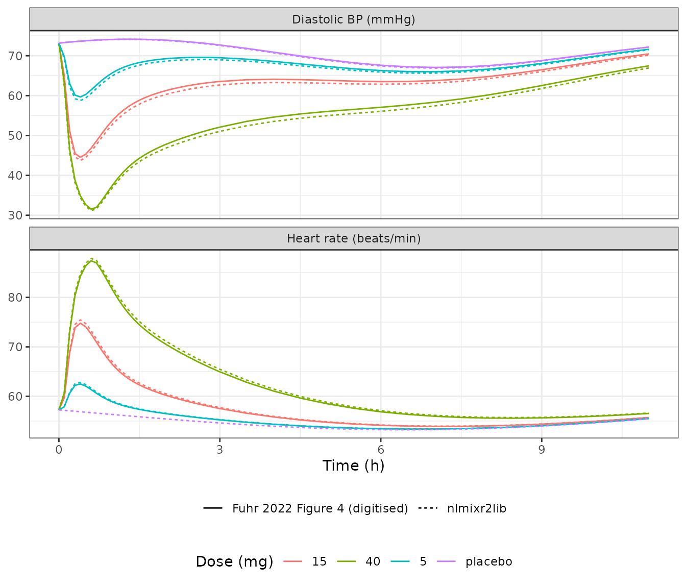
Replicates Figure 4 panels d and g of Fuhr 2022.
The packaged model reproduces the paper’s DBP curves to within about
1 mmHg and its HR curves to within about 0.7 beats/min. The DBP curves
carry a small systematic offset (the packaged model predicts slightly
more decrease) that is absent from the placebo curve, so it comes from
the drug term. The likely cause is rounding: Table 3 prints EC50 as
0.04 umol/L. Refitting EC50 to the digitised curves with
Emax held at 56.18 gives about 0.044 umol/L, inside the rounding
interval 0.035-0.045. The maintainers did not adjust any value; the
printed parameters are packaged as published. The same refit for HR
recovers h = 1.40, EC50 = 0.052 umol/L and Emax = 39.6
beats/min, all consistent with Table 3. Using h = 1.4 for
DBP as well would make the DBP curves miss by up to 4.5 mmHg. That
supports reading Table 3 as having no Hill coefficient for DBP (h =
1).
# Deterministic: the only differences are digitisation error and the 2-dp
# rounding of EC50. Measured maxima 1.10 mmHg (DBP) and 0.67 bpm (HR). A
# wrong Hill coefficient (h = 1.4 for DBP) gives 4.5 mmHg, and a
# percent-vs-fraction slip on an amplitude gives tens of mmHg.
stopifnot(
  max(abs(cmp_edgar$dbp_diff)) < 2,
  max(abs(cmp_edgar$dbp_diff[cmp_edgar$arm == "placebo"])) < 0.5,
  sum(!is.na(cmp_edgar$hr_diff)) == 3 * nrow(edgar), # three dosed HR arms
  max(abs(cmp_edgar$hr_diff), na.rm = TRUE) < 1.5
)
Hypertensive patients: Blychert 1990 and Hedner 1986 (panels e, f, h, i)
Panels b and c (the plasma concentrations for these two studies) are raster images, so the drug curves cannot be driven from a digitised concentration. Two checks remain:
-
Placebo curves, which depend only on the circadian
layer and the Table S5 parameters (
CEFFECT = 0). - Cross-endpoint consistency. The drug-minus-placebo DBP difference of panel e (or f) is inverted through the DBP Emax function to the plasma concentration it implies. That concentration then drives the HR model, and the result is compared with the drug HR curve of panel h (or i). This tests whether the DBP and HR curves come from one concentration through the Table 3 Emax parameters, and whether hypertensive patients share those parameters.
check_ht <- function(dig, study_mod, study) {
  e_dbp <- pmax(dig$dbp_placebo - dig$dbp_drug, 0)
  conc_implied <- 0.04 * e_dbp / (56.18 - e_dbp) # umol/L, inverse of Eq. S20
  ev <- bind_rows(
    data.frame(id = 1L, time = dig$time, CEFFECT = 0),
    data.frame(id = 2L, time = dig$time, CEFFECT = conc_implied)
  ) |>
    # DIS_HYPERT stays 0: the study-specific Table S5 means passed to
    # study_model() already are the hypertensive values, and setting it to 1
    # would apply the Table 3 hypertensive ratio on top of them.
    mutate(evid = 0, amt = 0, DIS_HYPERT = 0)
  sim <- as.data.frame(rxSolve(study_mod, ev))
  stopifnot(nrow(sim) == 2 * nrow(dig))
  data.frame(
    study = study,
    time = dig$time,
    conc_implied_ngmL = conc_implied * mw,
    dbp_placebo_paper = dig$dbp_placebo,
    dbp_placebo = sim$dbp[sim$id == 1],
    hr_placebo_paper = dig$hr_placebo,
    hr_placebo = sim$hr[sim$id == 1],
    hr_drug_paper = dig$hr_drug,
    hr_drug = sim$hr[sim$id == 2]
  )
}
cmp_ht <- bind_rows(
  check_ht(blychert, mod_blychert, "Blychert 1990"),
  check_ht(hedner, mod_hedner, "Hedner 1986")
)
#> Warning: multi-subject simulation without without 'omega'
#> Warning: multi-subject simulation without without 'omega'
ht_summary <- cmp_ht |>
  group_by(study) |>
  summarise(
    `Placebo DBP max abs diff (mmHg)` = max(abs(dbp_placebo - dbp_placebo_paper)),
    `Placebo HR max abs diff (bpm)` = max(abs(hr_placebo - hr_placebo_paper)),
    `Drug HR max abs diff (bpm)` = max(abs(hr_drug - hr_drug_paper)),
    `Implied peak conc (ng/mL)` = max(conc_implied_ngmL),
    .groups = "drop"
  ) |>
  rename(Study = study)
knitr::kable(ht_summary, digits = 2)| Study | Placebo DBP max abs diff (mmHg) | Placebo HR max abs diff (bpm) | Drug HR max abs diff (bpm) | Implied peak conc (ng/mL) |
|---|---|---|---|---|
| Blychert 1990 | 0.26 | 0.01 | 0.26 | 7.83 |
| Hedner 1986 | 0.25 | 0.01 | 0.26 | 6.74 |
# Deterministic. Measured maxima: placebo DBP 0.26 mmHg, placebo HR 0.01 bpm,
# drug HR 0.26 bpm.
stopifnot(
  all(ht_summary$`Placebo DBP max abs diff (mmHg)` < 0.5),
  all(ht_summary$`Placebo HR max abs diff (bpm)` < 0.5),
  all(ht_summary$`Drug HR max abs diff (bpm)` < 1)
)
cmp_ht |>
  select(study, time, dbp_placebo, dbp_placebo_paper, hr_placebo, hr_placebo_paper, hr_drug, hr_drug_paper) |>
  pivot_longer(-c(study, time)) |>
  mutate(
    source = ifelse(grepl("paper", name), "Fuhr 2022 Figure 4 (digitised)", "nlmixr2lib"),
    curve = sub("_paper", "", name)
  ) |>
  ggplot(aes(time, value, colour = curve, linetype = source)) +
  geom_line() +
  facet_wrap(~study, scales = "free", ncol = 1) +
  labs(x = "Time (h)", y = "mmHg or beats/min", colour = NULL, linetype = NULL) +
  theme_bw() +
  theme(legend.position = "bottom", legend.box = "vertical")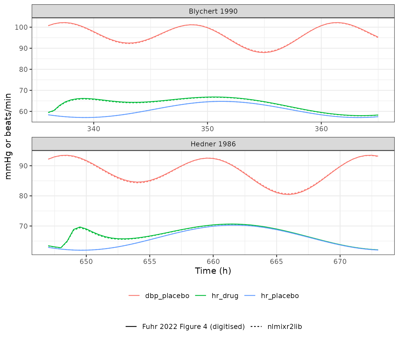
Replicates the placebo curves of Figure 4 panels e, f, h and i, and the drug curves of panels h and i using the concentration implied by panels e and f. The implied peak concentrations (about 7.8 ng/mL for Blychert 1990 and 6.7 ng/mL for Hedner 1986) agree with the predicted peaks shown in panels b and c (about 8 and 7 ng/mL). Both checks pass: the circadian layer is reproduced exactly, and the DBP and HR models are mutually consistent in hypertensive patients with the shared Table 3 Emax parameters.
Non-compartmental analysis
Not applicable. The packaged model has no PK layer and no dose
records: felodipine concentration is an input (CEFFECT),
and the paper reports no NCA of the PD endpoints. The deterministic
checks and the Figure 4 replication above take the place of the PKNCA
comparison.
Assumptions and deviations
-
PD layer only. The PK-Sim / MoBi whole-body PBPK
layer (Table 2) is not reproduced, because its organ volumes, blood
flows, partition coefficients and CYP3A4 expression profile are platform
database outputs the paper does not print. The felodipine plasma
concentration must be supplied as
CEFFECTin umol/L. Divide ng/mL by 384.25 (Table 2 molecular weight), or nmol/L by 1000. The DDI scenarios of the paper (Section 3.3) act through the PBPK layer. With this model they are reproduced only by supplying the DDI-altered plasma concentrations. -
Hill coefficient for DBP. Equation 1 / S20 is
written with a Hill coefficient
h, but Table 3 and Table S6 listhfor the HR model only. The DBP Emax function is therefore hyperbolic (h = 1). The Figure 4 replication above supports this reading: h = 1 reproduces panel d to within about 1 mmHg, h = 1.4 misses by up to 4.5 mmHg. -
Amplitudes are fractions. Table 3 reports the
amplitudes in percent (2.14 %, 5.93 %, 6.3 %). Equations S17 and S19
multiply the 24 h mean by
(1 + circ), so they are entered as fractions (0.0214, 0.0593, 0.063). The exact match to the placebo curves confirms the scale. -
Time origin of the phases. Fuhr 2022 optimised the
circadian phases against each study’s own simulation time (Figure 4 time
axes run from the first dose, e.g. 336-366 h for day 15).
timein this model is that simulation clock in hours, and the phases are relative to its origin, not to midnight. The published phases are not clock times. The Table 3 typical phases (5.28 h, 0.16 h and 11.8 h) are means over studies whose dosing clock times differed, so they describe a generic study only. To reproduce a specific study, override them with its Table S5 values, as done above. - Study-specific circadian parameters. The 24 h means and phases were re-optimised for every simulated study (Table S5); Table 3 reports their means (SD). The packaged typical values are the Table 3 means. The SDs (e.g. 6.76 mmHg for BPmean) describe between-study spread of the optimised values, not between-subject variability, and are not encoded as random effects. The Table 3 means could not be recomputed exactly from the Table S5 rows (for example, the healthy-volunteer BPmean rows average 70.9 mmHg against the printed 70.4 mmHg), probably because the summary also covers simulations not listed in Table S5. The printed Table 3 values are used.
-
Hypertension. Table 3 gives separate 24 h means for
healthy and hypertensive individuals (footnote b). These are encoded
through the
DIS_HYPERTindicator as log-ratio shifts that reproduce the printed values exactly. The paper also reduced CYP3A4 kcat by 32 % on average in hypertensive individuals (Results 3.1). That is a PBPK-layer effect and reaches this model only throughCEFFECT. -
No variability. No inter-individual variability and
no residual-error model are reported. Both are zero
(
addSd_dbpandaddSd_hrfixed at 0), so the model gives typical-value predictions of mean DBP and HR. - No tolerance. The paper notes that HR tolerance during multiple dosing could not be modelled for lack of data (Discussion). The HR effect is therefore the same on every dosing day.
- Systolic blood pressure was not modelled by the paper (Discussion).
- Digitisation. The Figure 4 curves were extracted from the article’s vector graphics, with each axis calibrated on its tick marks. Digitisation error is a small fraction of 1 mmHg / 1 beat per minute, judged by the 0.01 bpm agreement on the HR placebo curves.