Glucarpidase rescue after high-dose methotrexate (Fukaya 2023)
Source:vignettes/articles/Fukaya_2023_glucarpidase.Rmd
Fukaya_2023_glucarpidase.RmdModel and source
- Citation: Fukaya Y, Kimura T, Hamada Y, Yoshimura K, Hiraga H, Yuza Y, Ogawa A, Hara J, Koh K, Kikuta A, Koga Y, Kawamoto H. Development of a population pharmacokinetics and pharmacodynamics model of glucarpidase rescue treatment after high-dose methotrexate therapy. Front Oncol. 2023;13:1003633. doi:10.3389/fonc.2023.1003633
- Article: https://doi.org/10.3389/fonc.2023.1003633 (open access)
- Supporting regulatory document for the activity-to-mass conversion and the Michaelis-Menten constant: EMA Voraxaze public assessment report (EMA/CHMP/751047/2021), https://www.ema.europa.eu/en/documents/assessment-report/voraxaze-epar-public-assessment-report_en.pdf
Fukaya et al. report two population models fitted in Phoenix NLME 7.0 (FOCE-ELS), and both are packaged:
-
Fukaya_2023_glucarpidase_healthy– one-compartment glucarpidase (CPG2) popPK in 16 healthy Japanese men (phase 1; 20 or 50 U/kg, repeated at 48 h). -
Fukaya_2023_glucarpidase_methotrexate– the phase 2 model in 15 patients with delayed methotrexate (MTX) excretion: one-compartment CPG2 PK coupled to two-compartment MTX PK in which CPG2 hydrolyses MTX by Michaelis-Menten kinetics withVmax = alpha * [CPG2].
mod_p1 <- rxode2::rxode2(readModelDb("Fukaya_2023_glucarpidase_healthy"))
#> ℹ parameter labels from comments will be replaced by 'label()'
mod_p2 <- rxode2::rxode2(readModelDb("Fukaya_2023_glucarpidase_methotrexate"))
#> ℹ parameter labels from comments will be replaced by 'label()'
Population
Phase 1 (healthy volunteers). Sixteen Japanese men, randomised 8 per arm to 20 or 50 U/kg glucarpidase as a 5-min IV infusion with an identical second dose 48 h later; mean age 24.9 years (20-40), height 169.6 cm (162.6-184.8), weight 60.9 kg (54.3-66.9); 192 plasma CPG2 concentrations (Fukaya 2023 Section 3.1).
Phase 2 (patients). Fifteen Japanese patients (9 male, 6 female) with delayed MTX excretion after high-dose MTX (median 8.0 g/m^2, range 2.9-14.3): osteosarcoma 9, acute lymphocytic leukaemia 3, non-Hodgkin lymphoma 2, medulloblastoma 1. Median age 15 years (1-75), height 156.0 cm (78.5-177.5), weight 47.0 kg (10.7-78.1), serum creatinine 0.81 mg/dL (0.23-3.47). Each received 50 U/kg glucarpidase within 12 h of confirmed delayed excretion, and a second dose if plasma MTX stayed above 1 umol/L more than 46 h later; 88 CPG2 and 115 MTX (HPLC) concentrations (Table 2, Section 3.1).
The same information is available programmatically via
readModelDb("Fukaya_2023_glucarpidase_methotrexate")()$population.
Source trace
| Equation / parameter | Value | Source location |
|---|---|---|
Phase 1 lcl (tvCL at BSA = 1) |
log(0.0590) L/h | Table 4, phase 1 |
Phase 1 e_bsa_cl
|
3.227 | Table 4, phase 1 (theta1) |
Phase 1 lvc (tvV at BSA = 1) |
log(0.957) L | Table 4, phase 1 |
Phase 1 e_bsa_vc
|
2.251 | Table 4, phase 1 (theta2) |
Phase 1 etalcl, etalvc
|
CV 3.2 %, 6.4 % | Table 4, phase 1 |
Phase 1 addSd
|
0.170 mg/L | Table 4, phase 1; Section 2.5 additive error |
Phase 2 lcl_cpg2, e_bsa_cl_cpg2
|
log(0.238) L/h, 1.440 | Table 4, phase 2 |
Phase 2 lvc_cpg2, e_bsa_vc_cpg2
|
log(1.200) L, 1.561 | Table 4, phase 2 |
Phase 2 etalcl_cpg2, etalvc_cpg2
|
CV 17.4 %, 22.1 % | Table 4, phase 2 |
Phase 2 addSd_cpg2
|
0.100 mg/L | Table 4, phase 2 |
lcl_renal: CLr = tvCLr x WT / Scr / 60 |
log(3.248) L/h | Table 4; Section 3.2.2 equation |
lvc: Vc = tvVc x WT / BSA |
log(0.386) L | Table 4; Section 3.2.2 equation |
lvp: Vp = tvVp x WT / 60 |
log(3.052) L | Table 4; Section 3.2.2 equation |
lq |
log(0.0778) L/h, held constant | Table 4; Section 3.2.2 (Fukuhara 2008 value) |
lalpha |
log(6.545e5) | Table 4 (reported as L/h) |
km_cpg2 |
86 umol/L, held constant | Table 4; Section 3.2.2 equation; EMA assessment report |
etalcl_renal, etalvc, etalvp,
etalalpha
|
CV 33.5 %, 29.1 %, 90.6 %, 79.8 % | Table 4 |
propSd |
1.414 | Table 4; Section 2.6 Cij = Cij* x (1 + eps)
|
| MTX ODEs |
dXc/dt = -(Kr + K12) Xc + K21 Xp - alpha [CPG2] [Xc]/(Km + [Xc]),
dXp/dt = K12 Xc - K21 Xp
|
Section 2.6 and Section 3.2.2 equations; Figure 2 |
| CPG2 ODE | one compartment, first-order elimination, IV infusion | Section 2.5, Section 3.2.1, Figure 2 |
| Micro-constants |
Kr = CLr / Vc, Q = K12 Vc = K21 Vp
|
Section 2.6 |
IIV is reported as CV % and encoded as
omega^2 = log(CV^2 + 1).
Unit conventions
MTX amounts are in umol (MW 454.44 g/mol), MTX concentrations in umol/L, as in the paper’s figures and the Michaelis-Menten constant. CPG2 concentrations are in mg/L, as in the paper’s CPG2 figures and residual error. The paper doses CPG2 in U/kg and does not state a U-to-mg factor. The EMA assessment report gives the same 50 U/kg study (PR001-CLN-005) in both activity and mass units – AUC0-tau 7.56-8.61 U h/mL against 17.3-19.7 ug h/mL, and Cmax 1.21-1.44 U/mL against 2.76-3.29 ug/mL – which is 2.29 ug per unit in every pairing. That factor converts the doses below.
mw_mtx <- 454.44 # g/mol
ug_per_unit <- 19.7 / 8.61 # EMA assessment report, normal-renal-function AUC0-tau
round(c(ug_per_unit = ug_per_unit, alt_cmax = 3.29 / 1.44, alt_auc = 17.3 / 7.56), 3)
#> ug_per_unit    alt_cmax     alt_auc
#>       2.288       2.285       2.288
cpg2_mg <- function(u_per_kg, wt) u_per_kg * wt * ug_per_unit / 1000
bsa_dubois <- function(wt, ht) 0.007184 * wt^0.425 * ht^0.725
Two consistency checks on that factor against Fukaya’s own data: at the phase 1 mean weight and typical V, 50 U/kg gives about 2.2 mg/L at the end of the infusion and 20 U/kg about 0.9 mg/L, which are the peak levels in Figure 3A-B.
Phase 1: healthy volunteers
Typical values against the reported post-hoc means
The paper reports post-hoc mean CL = 0.329 L/h and V = 3.17 L for phase 1 (Section 3.2.1), and the same as 0.0896 mL/min/kg and 51.9 mL/kg (Discussion). The model is un-normalised in BSA, so the typical value at the cohort mean BSA should land on them. The paper does not name its BSA formula; DuBois is used.
bsa_p1 <- bsa_dubois(60.9, 169.6)
cl_p1 <- 0.0590 * bsa_p1^3.227
v_p1 <- 0.957 * bsa_p1^2.251
p1_check <- data.frame(
  Quantity = c("CL (L/h)", "V (L)", "CL (mL/min/kg)", "V (mL/kg)"),
  Model = c(cl_p1, v_p1, cl_p1 / 60.9 * 1000 / 60, v_p1 / 60.9 * 1000),
  Paper = c(0.329, 3.17, 0.0896, 51.9)
) |>
  mutate(`% diff` = 100 * (Model - Paper) / Paper)
knitr::kable(p1_check, digits = c(0, 4, 4, 2))| Quantity | Model | Paper | % diff |
|---|---|---|---|
| CL (L/h) | 0.3287 | 0.3290 | -0.09 |
| V (L) | 3.1715 | 3.1700 | 0.05 |
| CL (mL/min/kg) | 0.0900 | 0.0896 | 0.40 |
| V (mL/kg) | 52.0764 | 51.9000 | 0.34 |
Virtual phase 1 cohort and VPC
set.seed(20230130)
rxode2::rxSetSeed(20230130)
n_per_arm <- 100
p1_cov <- data.frame(id = seq_len(2 * n_per_arm)) |>
  mutate(
    treatment = rep(c("20 U/kg", "50 U/kg"), each = n_per_arm),
    u_per_kg = rep(c(20, 50), each = n_per_arm),
    WT = pmin(pmax(rnorm(n(), 60.9, 3.5), 54.3), 66.9),
    HT = pmin(pmax(rnorm(n(), 169.6, 5.5), 162.6), 184.8),
    BSA = bsa_dubois(WT, HT),
    dose_mg = cpg2_mg(u_per_kg, WT)
  )
obs_t <- sort(unique(c(
  0, 5 / 60, 0.25, 0.5, 1, 2, 4, 8, 12, 24, 36, 47.99,
  48 + c(5 / 60, 0.25, 0.5, 1, 2, 4, 8, 12, 24, 36, 48)
)))
p1_ev <- bind_rows(
  p1_cov |> mutate(time = 0, amt = dose_mg, dur = 5 / 60, evid = 1),
  p1_cov |> mutate(time = 48, amt = dose_mg, dur = 5 / 60, evid = 1),
  tidyr::crossing(p1_cov, time = obs_t) |> mutate(amt = 0, dur = 0, evid = 0)
) |>
  mutate(cmt = "central") |>
  select(id, time, amt, dur, evid, cmt, treatment, WT, BSA) |>
  arrange(id, time, desc(evid))
p1_sim <- rxode2::rxSolve(mod_p1, p1_ev, returnType = "data.frame",
                          keep = "treatment")
p1_sim |>
  filter(time > 0) |>
  group_by(treatment, time) |>
  summarise(
    p05 = quantile(sim, 0.05), p50 = median(sim), p95 = quantile(sim, 0.95),
    .groups = "drop"
  ) |>
  ggplot(aes(time, p50)) +
  geom_ribbon(aes(ymin = p05, ymax = p95), fill = "steelblue", alpha = 0.3) +
  geom_line() +
  facet_wrap(~treatment) +
  labs(x = "Time after first CPG2 dose (h)", y = "Plasma CPG2 (mg/L)")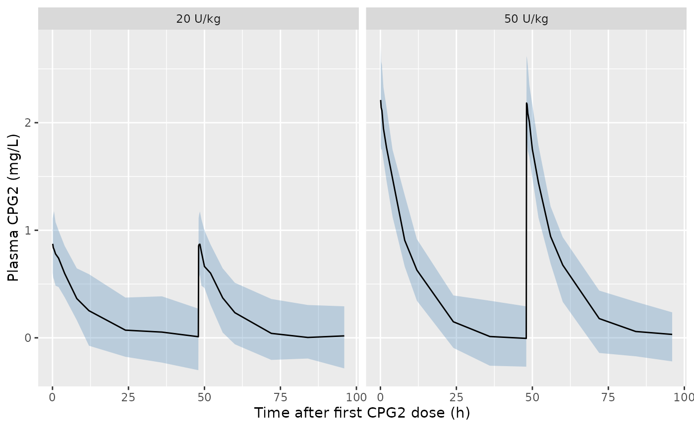
Replicates Figure 5A and Figure 3A-B of Fukaya 2023: simulated phase 1 CPG2 concentrations (median and 5th-95th percentiles, 100 virtual subjects per arm, residual error included).
PKNCA on the first dosing interval
p1_conc <- p1_sim |>
  filter(!is.na(Cc), time <= 48) |>
  select(id, time, Cc, treatment)
p1_dose <- p1_ev |>
  filter(evid == 1, time == 0) |>
  select(id, time, amt, dur, treatment)
p1_nca <- PKNCA::pk.nca(PKNCA::PKNCAdata(
  PKNCA::PKNCAconc(p1_conc, Cc ~ time | treatment + id),
  PKNCA::PKNCAdose(p1_dose, amt ~ time | treatment + id, duration = "dur"),
  intervals = data.frame(
    start = 0, end = Inf, cmax = TRUE, half.life = TRUE,
    aucinf.obs = TRUE, cl.obs = TRUE, vz.obs = TRUE
  )
))
p1_nca_sum <- as.data.frame(p1_nca$result) |>
  filter(PPTESTCD %in% c("cmax", "half.life", "aucinf.obs", "cl.obs", "vz.obs")) |>
  group_by(treatment, PPTESTCD) |>
  summarise(median = median(PPORRES), .groups = "drop") |>
  tidyr::pivot_wider(names_from = PPTESTCD, values_from = median)
p1_nca_sum |>
  dplyr::rename(
    Treatment = treatment, `Cmax (mg/L)` = cmax, `t1/2 (h)` = half.life,
    `AUC0-inf (mg h/L)` = aucinf.obs, `CL (L/h)` = cl.obs, `Vz (L)` = vz.obs
  ) |>
knitr::kable(digits = 3)| Treatment | AUC0-inf (mg h/L) | CL (L/h) | Cmax (mg/L) | t1/2 (h) | Vz (L) |
|---|---|---|---|---|---|
| 20 U/kg | 8.488 | 0.332 | 0.868 | 6.689 | 3.225 |
| 50 U/kg | 20.875 | 0.335 | 2.186 | 6.620 | 3.133 |
Fukaya 2023 quotes the earlier non-compartmental analysis of the same phase 1 study as CL = 0.291-0.347 L/h and V = 3.12-3.67 L (Discussion, reference 15). The interval is reported without saying which end belongs to which dose group, so the table compares the simulated median of each arm with the whole interval.
p1_vs_paper <- p1_nca_sum |>
  transmute(
    treatment,
    cl = cl.obs, cl_in_range = cl.obs >= 0.291 & cl.obs <= 0.347,
    vz = vz.obs, vz_in_range = vz.obs >= 3.12 & vz.obs <= 3.67
  )
p1_vs_paper |>
  dplyr::rename(
    Treatment = treatment, `Simulated CL (L/h)` = cl,
    `Within 0.291-0.347` = cl_in_range, `Simulated Vz (L)` = vz,
    `Within 3.12-3.67` = vz_in_range
  ) |>
knitr::kable(digits = 3)| Treatment | Simulated CL (L/h) | Within 0.291-0.347 | Simulated Vz (L) | Within 3.12-3.67 |
|---|---|---|---|---|
| 20 U/kg | 0.332 | TRUE | 3.225 | TRUE |
| 50 U/kg | 0.335 | TRUE | 3.133 | TRUE |
Phase 2: glucarpidase and methotrexate in patients
Typical values against the reported post-hoc means
The paper reports phase 2 post-hoc means for CPG2 (CL 0.380 L/h, V 2.04 L, Section 3.2.1) and MTX (CLr 2.424 L/h, Vc 12.6 L, Vp 2.15 L, alpha 8.131e5, Section 3.2.2). Individual covariates are not published, so the table uses a typical patient at the Table 2 median weight and height. The MTX renal clearance is shown at the baseline median serum creatinine (0.81 mg/dL) and at the mean measured just before CPG2 (1.23 mg/dL, Discussion), since the post-hoc mean should fall between the two.
wt_med <- 47
bsa_med <- bsa_dubois(wt_med, 156)
omega_alpha <- log(0.798^2 + 1)
p2_check <- data.frame(
  Quantity = c(
    "CPG2 CL (L/h)", "CPG2 V (L)", "MTX Vc (L)", "MTX Vp (L)",
    "MTX CLr at Scr 0.81 (L/h)", "MTX CLr at Scr 1.23 (L/h)",
    "alpha, lognormal mean"
  ),
  Model = c(
    0.238 * bsa_med^1.440, 1.200 * bsa_med^1.561,
    0.386 * wt_med / bsa_med, 3.052 * wt_med / 60,
    3.248 * wt_med / 0.81 / 60, 3.248 * wt_med / 1.23 / 60,
    6.545e5 * exp(omega_alpha / 2)
  ),
  Paper = c(0.380, 2.04, 12.6, 2.15, 2.424, 2.424, 8.131e5)
) |>
  mutate(`% diff` = 100 * (Model - Paper) / Paper)
knitr::kable(p2_check, digits = 3)| Quantity | Model | Paper | % diff |
|---|---|---|---|
| CPG2 CL (L/h) | 0.401 | 3.800e-01 | 5.416 |
| CPG2 V (L) | 2.110 | 2.040e+00 | 3.434 |
| MTX Vc (L) | 12.638 | 1.260e+01 | 0.298 |
| MTX Vp (L) | 2.391 | 2.150e+00 | 11.197 |
| MTX CLr at Scr 0.81 (L/h) | 3.141 | 2.424e+00 | 29.582 |
| MTX CLr at Scr 1.23 (L/h) | 2.069 | 2.424e+00 | -14.665 |
| alpha, lognormal mean | 837351.861 | 8.131e+05 | 2.983 |
The CPG2 values and MTX Vc fall within 6 % of the post-hoc means, MTX
Vp is 11 % above, and the MTX CLr post-hoc mean falls between the two
serum-creatinine anchors. The lognormal mean of alpha,
tv * exp(omega^2 / 2) with
omega^2 = log(CV^2 + 1), is within 3 % of the reported
post-hoc mean, which supports reading the Table 4 CV % values as
lognormal IIV.
Typical patient: depletion and rebound
The scenario below is illustrative: the paper does not give each patient’s MTX infusion schedule or the time from the MTX start to glucarpidase. A typical patient (47 kg, 156 cm, serum creatinine 1.23 mg/dL) receives 8 g/m^2 MTX over 4 h, then 50 U/kg glucarpidase over 5 min at 40 h.
t_cpg2 <- 40
make_p2_events <- function(cov, t_cpg2) {
  obs_t <- sort(unique(c(
    seq(0, t_cpg2 + 96, by = 1), t_cpg2 - 0.01,
    t_cpg2 + c(5 / 60, 0.25, 1 / 3, 0.5, 2, 6, 24, 48)
  )))
  bind_rows(
    cov |> mutate(time = 0, amt = mtx_umol, dur = 4, evid = 1, cmt = "central"),
    cov |> mutate(time = t_cpg2, amt = cpg2_dose, dur = 5 / 60, evid = 1,
                  cmt = "central_cpg2"),
    tidyr::crossing(cov, time = obs_t) |>
      mutate(amt = 0, dur = 0, evid = 0, cmt = "Cc")
  ) |>
    select(id, time, amt, dur, evid, cmt, everything()) |>
    select(-mtx_umol, -cpg2_dose) |>
    arrange(id, time, desc(evid))
}
typ_cov <- data.frame(id = 1, WT = wt_med, BSA = bsa_med, CREAT = 1.23) |>
  mutate(mtx_umol = 8 * BSA * 1e6 / mw_mtx, cpg2_dose = cpg2_mg(50, WT))
typ_ev <- make_p2_events(typ_cov, t_cpg2)
typ_sim <- rxode2::rxSolve(mod_p2, typ_ev, omega = NA, sigma = NA,
                           useLinCmt = FALSE, returnType = "data.frame")
# The state order is fixed by the d/dt() lines; observing the declared
# endpoint `Cc` must not have renumbered it.
stopifnot(identical(mod_p2$state, c("central", "peripheral1", "central_cpg2")))
typ_sim |>
  select(time, MTX = Cc, CPG2 = Cc_cpg2) |>
  tidyr::pivot_longer(-time, names_to = "analyte", values_to = "conc") |>
  filter(conc > 1e-4) |>
  ggplot(aes(time - t_cpg2, conc)) +
  geom_line() +
  geom_hline(
    data = data.frame(analyte = "MTX", y = c(0.1, 1)),
    aes(yintercept = y), linetype = "dashed"
  ) +
  scale_y_log10() +
  facet_wrap(~analyte, scales = "free_y", ncol = 1,
             labeller = as_labeller(c(MTX = "MTX (umol/L)", CPG2 = "CPG2 (mg/L)"))) +
  labs(x = "Time after first CPG2 dose (h)", y = "Concentration")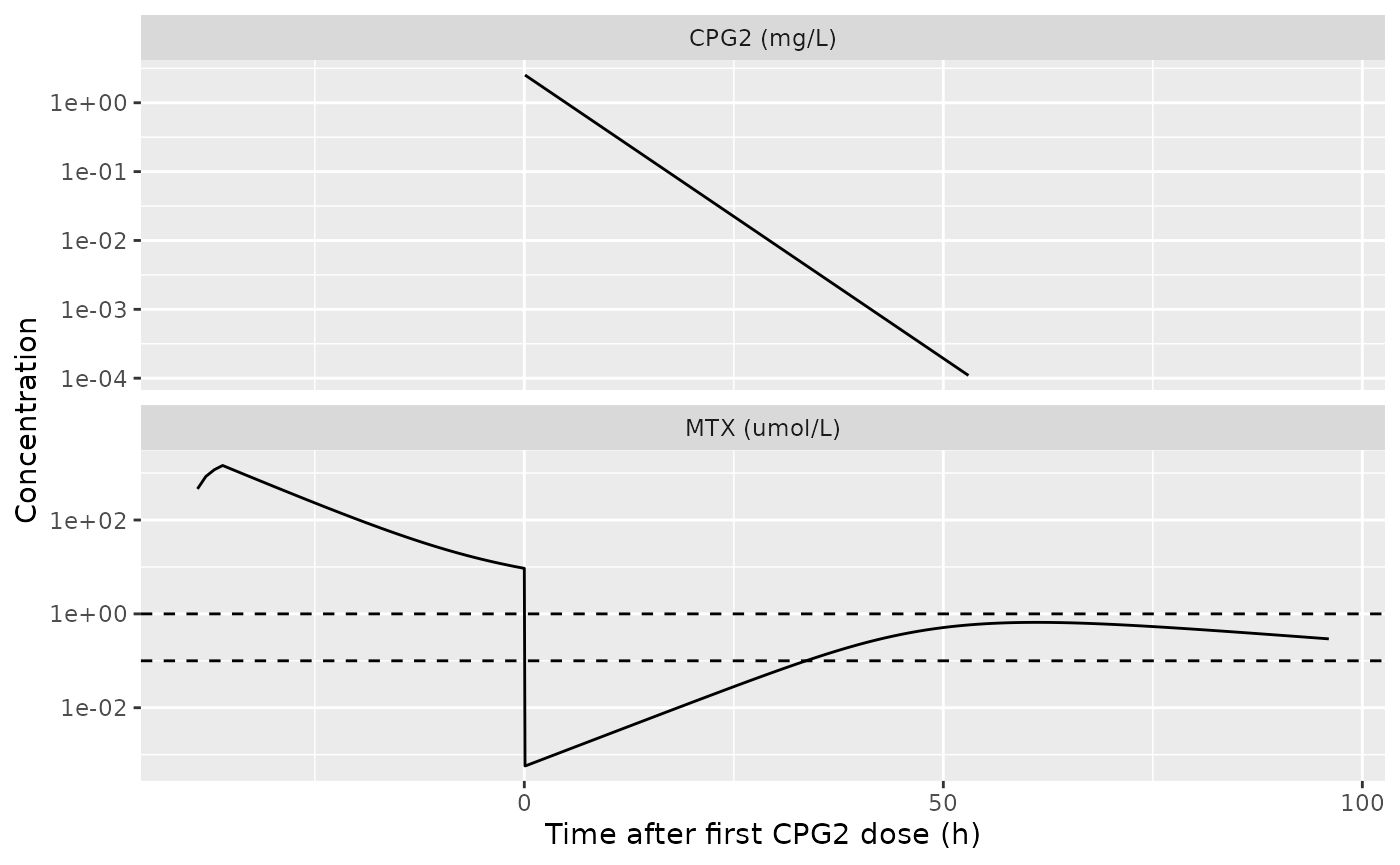
Typical-patient MTX and CPG2 concentrations; compare the individual MTX profiles of Figure 6 of Fukaya 2023 (rapid fall after CPG2 followed by a rebound). Dashed lines mark 0.1 and 1 umol/L.
at <- function(t) typ_sim$Cc[which.min(abs(typ_sim$time - t))]
typ_tab <- data.frame(
  `Time after CPG2` = c("pre-dose", "15 min", "6 h", "24 h", "48 h"),
  `MTX (umol/L)` = c(at(t_cpg2 - 0.01), at(t_cpg2 + 0.25), at(t_cpg2 + 6),
                     at(t_cpg2 + 24), at(t_cpg2 + 48)),
  check.names = FALSE
)
knitr::kable(typ_tab, digits = 4)| Time after CPG2 | MTX (umol/L) |
|---|---|
| pre-dose | 9.3379 |
| 15 min | 0.0006 |
| 6 h | 0.0014 |
| 24 h | 0.0241 |
| 48 h | 0.4559 |
At typical values, CPG2 drives MTX down by more than three orders of magnitude, and the rebound builds over the next 1-3 days as MTX returns from the peripheral compartment while CPG2 is cleared. The individual Bayesian predictions in Figure 6 bottom out higher, around 0.01-1 umol/L, and rebound sooner. The authors note the same limitation: the model underestimates MTX concentrations at early times after CPG2 (Discussion).
Virtual phase 2 cohort
set.seed(20230131)
rxode2::rxSetSeed(20230131)
n_p2 <- 200
p2_cov <- data.frame(id = seq_len(n_p2)) |>
  mutate(
    WT = exp(pmin(pmax(rnorm(n(), log(47), 0.45), log(10.7)), log(78.1))),
    BMI = pmin(pmax(rnorm(n(), 19.5, 2.5), 15), 26),
    HT = 100 * sqrt(WT / BMI),
    BSA = bsa_dubois(WT, HT),
    CREAT = exp(pmin(pmax(rnorm(n(), log(1.0), 0.5), log(0.23)), log(3.47))),
    mtx_umol = 8 * BSA * 1e6 / mw_mtx,
    cpg2_dose = cpg2_mg(50, WT)
  ) |>
  select(-BMI, -HT)
p2_ev <- make_p2_events(p2_cov, t_cpg2)
p2_sim <- rxode2::rxSolve(mod_p2, p2_ev, useLinCmt = FALSE,
                          returnType = "data.frame")
The paper reports that glucarpidase lowers plasma MTX by more than 95
% within 15 min (Introduction; the EMA assessment report gives a 97-99 %
median within 15 min across four clinical studies), and that every
patient had a rebound (Discussion). The checks below use the individual
predictions (Cc, no residual error), because a 141 %
proportional residual error would hide the structural behaviour.
p2_ind <- p2_sim |>
  group_by(id) |>
  summarise(
    pre = Cc[which.min(abs(time - (t_cpg2 - 0.01)))],
    post15 = Cc[which.min(abs(time - (t_cpg2 + 0.25)))],
    post2h = Cc[which.min(abs(time - (t_cpg2 + 2)))],
    peak_after = max(Cc[time > t_cpg2 + 2 & time <= t_cpg2 + 96]),
    c48 = Cc[which.min(abs(time - (t_cpg2 + 48)))],
    .groups = "drop"
  ) |>
  mutate(
    pct_reduction_15min = 100 * (1 - post15 / pre),
    rebound = peak_after > post2h
  )
p2_summary <- data.frame(
  Check = c(
    "Median % reduction 15 min after CPG2",
    "10th percentile of % reduction at 15 min",
    "Fraction of subjects with a rebound",
    "Fraction above 1 umol/L at 48 h after CPG2"
  ),
  Simulated = c(
    median(p2_ind$pct_reduction_15min),
    quantile(p2_ind$pct_reduction_15min, 0.1),
    mean(p2_ind$rebound),
    mean(p2_ind$c48 > 1)
  ),
  Paper = c("> 95 % (97-99 % median, EMA)", "", "all 15 patients", "2 of 15")
)
knitr::kable(p2_summary, digits = 3)| Check | Simulated | Paper |
|---|---|---|
| Median % reduction 15 min after CPG2 | 99.994 | > 95 % (97-99 % median, EMA) |
| 10th percentile of % reduction at 15 min | 99.970 | |
| Fraction of subjects with a rebound | 0.970 | all 15 patients |
| Fraction above 1 umol/L at 48 h after CPG2 | 0.125 | 2 of 15 |
# Robust quantiles and fractions, not cohort extremes.
stopifnot(
  median(p2_ind$pct_reduction_15min) > 95,
  quantile(p2_ind$pct_reduction_15min, 0.1) > 90,
  mean(p2_ind$rebound) > 0.9
)
p2_sim |>
  filter(time >= t_cpg2 - 1) |>
  group_by(time) |>
  summarise(
    p05 = quantile(Cc, 0.05), p50 = median(Cc), p95 = quantile(Cc, 0.95),
    .groups = "drop"
  ) |>
  ggplot(aes(time - t_cpg2, p50)) +
  geom_ribbon(aes(ymin = pmax(p05, 1e-4), ymax = p95), fill = "steelblue",
              alpha = 0.3) +
  geom_line() +
  geom_hline(yintercept = c(0.1, 1), linetype = "dashed") +
  scale_y_log10() +
  labs(x = "Time after first CPG2 dose (h)", y = "Plasma MTX (umol/L)")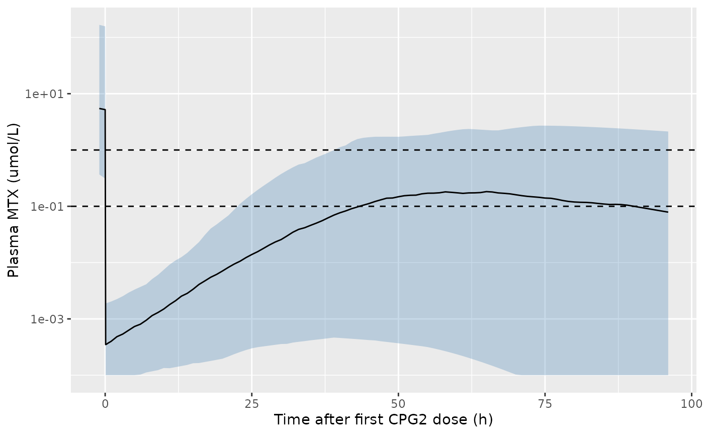
Simulated MTX after the first CPG2 dose in the virtual phase 2 cohort (median and 5th-95th percentiles of individual predictions); compare Figure 6 of Fukaya 2023.
PKNCA on glucarpidase in patients
p2_conc <- p2_sim |>
  filter(!is.na(Cc_cpg2), time >= t_cpg2) |>
  mutate(time = time - t_cpg2, treatment = "50 U/kg (patients)") |>
  select(id, time, Cc_cpg2, treatment)
p2_dose <- p2_ev |>
  filter(evid == 1, cmt == "central_cpg2") |>
  mutate(time = time - t_cpg2, treatment = "50 U/kg (patients)") |>
  select(id, time, amt, dur, treatment)
p2_nca <- PKNCA::pk.nca(PKNCA::PKNCAdata(
  PKNCA::PKNCAconc(p2_conc, Cc_cpg2 ~ time | treatment + id),
  PKNCA::PKNCAdose(p2_dose, amt ~ time | treatment + id, duration = "dur"),
  intervals = data.frame(
    start = 0, end = Inf, cmax = TRUE, half.life = TRUE,
    aucinf.obs = TRUE, cl.obs = TRUE
  )
))
#> Warning in assert_conc(conc, any_missing_conc = any_missing_conc): Negative
#> concentrations found
#> Warning in assert_conc(conc = conc): Negative concentrations found
#> Warning in assert_conc(conc, any_missing_conc = any_missing_conc): Negative
#> concentrations found
#> Warning in assert_conc(conc, any_missing_conc = any_missing_conc): Negative
#> concentrations found
#> Warning in assert_conc(conc, any_missing_conc = any_missing_conc): Negative
#> concentrations found
#> Warning in assert_conc(conc, any_missing_conc = any_missing_conc): Negative
#> concentrations found
#> Warning in assert_conc(conc, any_missing_conc = any_missing_conc): Negative
#> concentrations found
#> Warning in log(data$conc): NaNs produced
#> Warning in assert_conc(conc, any_missing_conc = any_missing_conc): Negative
#> concentrations found
p2_nca_kg <- as.data.frame(p2_nca$result) |>
  filter(PPTESTCD == "cl.obs") |>
  left_join(p2_cov |> select(id, WT), by = "id") |>
  mutate(cl_ml_min_kg = PPORRES * 1000 / 60 / WT)
summary(p2_nca)
#>  start end          treatment   N        cmax   half.life  aucinf.obs
#>      0 Inf 50 U/kg (patients) 200 2.55 [25.2] 3.83 [1.15] 13.7 [19.2]
#>        cl.obs
#>  0.357 [54.7]
#>
#> Caption: cmax, aucinf.obs, cl.obs: geometric mean and geometric coefficient of variation; half.life: arithmetic mean and standard deviation; N: number of subjects
The simulated geometric-mean CPG2 clearance in patients is close to the reported post-hoc mean of 0.380 L/h. The Discussion also gives phase 2 per-kg values (CL 0.0822 mL/min/kg, Vd 56.0 mL/kg) that do not agree with the paper’s own post-hoc means: at the median weight of 47 kg they correspond to 0.23 L/h and 2.6 L. Their ratio, V/CL = 11.4 h, also differs from the 5.4 h of the post-hoc means (2.04 L / 0.380 L/h). The phase 1 per-kg values do agree with the model (see above). The virtual-cohort mean here is 0.142 mL/min/kg, consistent with the post-hoc means and not with the per-kg figure.
Assumptions and deviations
- Two stages combined. The authors fitted CPG2 popPK first and fixed each patient’s post-hoc CPG2 CL and V when fitting the MTX model. The packaged phase 2 model simulates both stages together, so CPG2 IIV propagates into the MTX profile.
-
Units of alpha. Table 4 labels alpha “L/h” and the
Methods describe
Vmax (mass/time) = [catalyst] x alpha. With the paper’s units (CPG2 in mg/L, MTX in umol and umol/L, Km = 86 umol/L) the numerical value acts as umol/h of MTX hydrolysed per mg/L of CPG2, which is how the model uses it. - U-to-mg conversion. Not given in the paper; 2.29 ug/U is taken from the EMA assessment report (see Unit conventions). It sets the CPG2 concentration scale and therefore when MTX rebounds, but not CPG2 CL or V.
- BSA formula. Not named in the paper; DuBois reproduces the phase 1 post-hoc means to within 1 %.
- Serum creatinine. The paper does not say whether it was time-varying; the virtual cohorts hold it constant per subject. The phase 2 serum-creatinine distribution (lognormal, median 1.0 mg/dL, truncated to 0.23-3.47) is assumed, as are the weight and BMI distributions used to build heights.
- MTX residual error. Table 4 prints the MTX residual variability as 1.414 with the proportional error model of Section 2.6; it is encoded as a proportional SD of 1.414 (141 %).
- Second glucarpidase dose. The rule “second dose if MTX > 1 umol/L more than 46 h after the first” is a clinical decision and is not encoded; add a second dose event to simulate it.
- MTX dosing schedule. Individual MTX infusion durations and the interval to glucarpidase are not published; the 4-h infusion and the 40-h interval are illustrative. The fraction of virtual patients above 1 umol/L at 48 h therefore depends on that scenario and is shown for description only, not as a check against the paper’s 2 of 15.
- Phase 2 per-kg CPG2 values. The Discussion’s phase 2 per-kg CL and Vd are inconsistent with the paper’s own post-hoc means (see the PKNCA section); the model follows Table 4.